Predicting the future with Gaussian processes

Introduction

I recently gave a short introduction to non-parametric models in machine learning. Searching around for a good data set to use I ended up settling on polling data for the 2016 US presidential election. Luckily, fivethirtyeight has the data available to the public and nicely format so that made it a lot easier to hit the greound running.

Non-parametric models are used when you don’t want to make strong assumptions about the underlying data. Imagine that we’re in a forest and we’re collecting the locations of a certain type of tree. We could maybe use a known distribution to describe this, but the relationship might be so complex that none really fits the bill. Non-parametric approaches such as kernel density estimation can then be used.

Similarly, we could have data such as traffic to a particular website over time. Again, we could use something like a polynomial regression model to capture this relationship, however this again might not be complex enough to describe the relationship. Here, we could use the non-parametric technique known as a Gaussian process, to capture this relationship.

Here we’re going to use kernel density estimation to estimate the distribution of polls in time and then use Gaussian processes to capture the polling trends in time and estimate the expected popular vote share and uncertainty at the time of the election.

import pandas as pd
import numpy as np
import matplotlib.pyplot as plt
%matplotlib inline
data = pd.read_csv("http://projects.fivethirtyeight.com/general-model/president_general_polls_2016.csv")
data.head()

	cycle	branch	type	matchup	forecastdate	state	startdate	enddate	pollster	grade	...	adjpoll_clinton	adjpoll_trump	adjpoll_johnson	adjpoll_mcmullin	multiversions	url	poll_id	question_id	createddate	timestamp
0	2016	President	polls-plus	Clinton vs. Trump vs. Johnson	11/6/16	U.S.	11/1/2016	11/4/2016	ABC News/Washington Post	A+	...	46.10899	41.63457	4.555536	NaN	NaN	http://abcnews.go.com/Politics/qualifications-...	48472	75960	11/6/16	23:31:10 6 Nov 2016
1	2016	President	polls-plus	Clinton vs. Trump vs. Johnson	11/6/16	U.S.	10/31/2016	11/4/2016	Ipsos	A-	...	42.71292	38.80288	6.624687	NaN	NaN	http://www.realclearpolitics.com/docs/2016/201...	48484	75984	11/6/16	23:31:10 6 Nov 2016
2	2016	President	polls-plus	Clinton vs. Trump vs. Johnson	11/6/16	U.S.	11/3/2016	11/5/2016	NBC News/Wall Street Journal	A-	...	43.54423	40.91608	5.148813	NaN	NaN	http://www.nbcnews.com/storyline/2016-election...	48480	75974	11/6/16	23:31:10 6 Nov 2016
3	2016	President	polls-plus	Clinton vs. Trump vs. Johnson	11/6/16	U.S.	11/1/2016	11/3/2016	Fox News/Anderson Robbins Research/Shaw & Comp...	A	...	46.33723	44.03186	4.789080	NaN	*	http://www.foxnews.com/politics/interactive/20...	48361	75811	11/4/16	23:31:10 6 Nov 2016
4	2016	President	polls-plus	Clinton vs. Trump vs. Johnson	11/6/16	Wisconsin	10/26/2016	10/31/2016	Marquette University	A	...	45.46722	40.99278	2.582904	NaN	NaN	https://twitter.com/MULawPoll	48095	75264	11/2/16	23:31:10 6 Nov 2016

5 rows × 27 columns

Table looks like it has a lot of columns so let’s look at them.

data.columns.values

array(['cycle', 'branch', 'type', 'matchup', 'forecastdate', 'state',
       'startdate', 'enddate', 'pollster', 'grade', 'samplesize',
       'population', 'poll_wt', 'rawpoll_clinton', 'rawpoll_trump',
       'rawpoll_johnson', 'rawpoll_mcmullin', 'adjpoll_clinton',
       'adjpoll_trump', 'adjpoll_johnson', 'adjpoll_mcmullin',
       'multiversions', 'url', 'poll_id', 'question_id', 'createddate',
       'timestamp'], dtype=object)

Let’s first look at the pollster column and see how many polls each pollster has performed.

data.pollster.value_counts()

Ipsos                                                         2670
Google Consumer Surveys                                       2073
SurveyMonkey                                                  1671
USC Dornsife/LA Times                                          357
Rasmussen Reports/Pulse Opinion Research                       354
CVOTER International                                           342
The Times-Picayune/Lucid                                       312
Public Policy Polling                                          264
YouGov                                                         222
Emerson College                                                204
Quinnipiac University                                          174
Morning Consult                                                171
Gravis Marketing                                               171
Marist College                                                 141
SurveyUSA                                                      117
Monmouth University                                            114
Remington                                                       99
CNN/Opinion Research Corp.                                      84
Fox News/Anderson Robbins Research/Shaw & Company Research      81
ABC News/Washington Post                                        78
IBD/TIPP                                                        75
Suffolk University                                              66
Greenberg Quinlan Rosner (Democracy Corps)                      57
University of New Hampshire                                     48
Dan Jones & Associates                                          45
Maine People's Resource Center                                  45
NBC News/Wall Street Journal                                    45
Siena College                                                   42
Mason-Dixon Polling & Research, Inc.                            39
Mitchell Research & Communications                              39
                                                              ...
Political Marketing International, Inc./Red Racing Horses        3
Basswood Research                                                3
University of Akron                                              3
Feldman Group                                                    3
Cygnal Political                                                 3
Middle Tennessee State University                                3
Braun Research                                                   3
Cole Hargrave Snodgrass & Associates                             3
Dartmouth College                                                3
Target Insyght                                                   3
Expedition Strategies                                            3
Centre College                                                   3
Hoffman Research Group                                           3
National Journal                                                 3
Utah Valley University                                           3
R.L. Repass & Partners                                           3
Behavior Research Center (Rocky Mountain)                        3
OnMessage Inc.                                                   3
Riley Research Associates                                        3
Southern Illinois University                                     3
University of Houston                                            3
Florida Southern College                                         3
Baruch College                                                   3
First Tuesday Strategies                                         3
University of Wyoming                                            3
Meredith College                                                 3
BK Strategies                                                    3
University of Mary Washington                                    3
Merrill Poll                                                     3
University of Arkansas                                           3
Name: pollster, dtype: int64

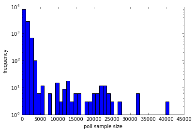
So there’s quite a spread. A few pollsters have performed polls many times and many have only done a few polls. Let’s plot a histogram of the distribution of polls

plt.hist(data.samplesize.dropna().values,bins=40);
plt.yscale('log');
plt.ylabel('frequency'); plt.xlabel('poll sample size');

Clean data

This next section we’ll clean the data to get it into a format suitable for doing some analysis

data.forecastdate = pd.to_datetime(data.forecastdate)
data.createddate = pd.to_datetime(data.createddate)

data['time2election'] = pd.to_datetime(data.createddate) - pd.datetime(2016,11,8)
data['time2election'] = data['time2election']/ np.timedelta64(1, 'D')

We’re only considering national polls so remove state-wide ones

national_data = data[data.state=='U.S.']

Remove NAs from poll date or sample size

national_data = national_data[np.isfinite(national_data.samplesize)]

Kernel density estimation of pollster times

First, let’s try and understand the distribution in time for the polls. We’ll do this by fitting a kernel density estimation to the time to election data.

from sklearn.neighbors import KernelDensity
from scipy.stats import norm

# Plot a 1D density example
N = 100
np.random.seed(1)
X = np.atleast_2d(data.time2election).T

X_plot = np.atleast_2d(np.linspace(X.min(), 0, 1000)).T
plt.figure(figsize=(18,8))



kde = KernelDensity(kernel='gaussian', bandwidth=5.0).fit(X)
log_dens = kde.score_samples(X_plot)
plt.plot(X_plot[:, 0], np.exp(log_dens), '-',
        label="kde estimate")


plt.legend(loc='upper left')
plt.plot(X[:, 0], -0.005 - 0.01 * np.random.random(X.shape[0]), '+k')

plt.xlim(X.min(), 0)
plt.ylim(-0.015, 0.02)
plt.grid()
plt.xlabel('time to election (days)')
plt.ylabel('density')
plt.show()

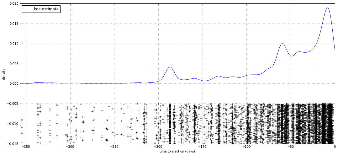
I’ve plotted the data below spread out along the y-axis so it’s easier to see. KDE does a good job at capturing the density of the polls. As expected, the number of polls are increasing towards the election, with a few interesting peaks that would be worth exploring.

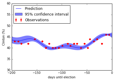
Predict popular vote using data from one pollster

Now, we’ll only look at one pollster to reduce data size as Gaussian processes can take a while to fit for many hundreds of points. The process can be repeated for all the pollsters to produce a prediction with confidence intervals for each of them. I decided on YouGov as it seemed fairly large.

national_data = national_data[national_data.pollster == 'YouGov']

Gaussian Process Regressor

Now we get into the main machine learning procedure. Scikit-learn has recently updated their Gaussian process library, so make sure you’re using version 0.18.1 or higher.

from sklearn.gaussian_process import GaussianProcessRegressor
from sklearn.gaussian_process.kernels import RBF, ConstantKernel as C

With the library loaded, let’s manipulate the data into the standard scikit-learn format. I’ve also standardised the polling by zeroing the mean, which is important for fitting as we will not be explicitly modelling the mean over time.

mpoll = np.mean(national_data.rawpoll_clinton)
sigpoll = 100.
p_clinton = np.array(national_data.rawpoll_clinton/sigpoll)
X = (np.atleast_2d(national_data.time2election).T).astype(float)
y = p_clinton - (mpoll)/sigpoll
#dy = 0.1*np.ones(len(y))/sigpoll#one point error
dy = p_clinton*(1-p_clinton)/national_data.samplesize.values

Scikit-learn gives a lot of flexibility in how we define the kernels. I settled on one that has a constant multiplied by a radial basis function, with values ranging from \(10^{-2}\) to 100 days.

#kernel = C(1.0, (1e-3, 1e3)) * RBF(7., (1e-2, 30.))
#kernel = 1.0 * RBF(length_scale=7.0, length_scale_bounds=(1e-2, 30.0))
kernel = C(1.0, (1e-3, 1e3)) * RBF(10, (1e-2, 1e2))

Now define the regressor. We’ve also produced a nugget or error based on the errors coming from a binomial distribution.

gp = GaussianProcessRegressor(kernel=kernel, alpha=(dy / y) ** 2,
                              n_restarts_optimizer=10)

gp.fit(X, y)  

GaussianProcessRegressor(alpha=array([  2.91595e-05,   3.03287e-05, ...,   3.15727e-05,   4.14705e-04]),
             copy_X_train=True, kernel=1**2 * RBF(length_scale=10),
             n_restarts_optimizer=10, normalize_y=False,
             optimizer='fmin_l_bfgs_b', random_state=None)

# Make the prediction on the meshed x-axis (ask for MSE as well)
x = np.atleast_2d(np.linspace(-250., 0, 1000)).T
y_pred, sigma = gp.predict(x, return_std=True)

# Plot the function, the prediction and the 95% confidence interval based on
# the MSE
fig = plt.figure()
py = sigpoll*y+mpoll
pdy = sigpoll*dy
py_pred = sigpoll*y_pred+mpoll
psigma = sigpoll*sigma
plt.errorbar(X.ravel(), py, pdy, fmt='r.', markersize=10, label=u'Observations')
plt.plot(x, py_pred, 'b-', label=u'Prediction')
plt.fill(np.concatenate([x, x[::-1]]),
         np.concatenate([py_pred - 1.9600 * psigma,
                        (py_pred + 1.9600 * psigma)[::-1]]),
         alpha=.5, fc='b', ec='None', label='95% confidence interval')
plt.xlabel('days until election')
plt.ylabel('Clinton (%)')
plt.ylim(30., 60.)
plt.xlim(-200.,0.)
plt.legend(loc='upper left')

plt.show()

Next Steps

With one nominee predicted, we’ll now predict the other in order to understand the uncertainty in the outcome of the election.

mpoll = np.mean(national_data.rawpoll_trump)
sigpoll = 100.
p_trump = np.array(national_data.rawpoll_trump/sigpoll)
Ty = p_trump - (mpoll)/sigpoll
#dy = 0.1*np.ones(len(y))/sigpoll#one point error
Tdy = (p_trump*(1-p_trump)/national_data.samplesize.values)

Tgp = GaussianProcessRegressor(kernel=kernel, alpha=(Tdy / Ty) ** 2,
                              n_restarts_optimizer=10)
Tgp.fit(X, Ty)  

GaussianProcessRegressor(alpha=array([  2.16801e-05,   7.77431e-05, ...,   4.36763e-05,   2.04680e-05]),
             copy_X_train=True, kernel=1**2 * RBF(length_scale=10),
             n_restarts_optimizer=10, normalize_y=False,
             optimizer='fmin_l_bfgs_b', random_state=None)

#Predict for Trump
Ty_pred, Tsigma = Tgp.predict(x, return_std=True)

# Plot the function, the prediction and the 95% confidence interval based on
# the MSE
fig = plt.figure(figsize=(18,8))
Tpy = sigpoll*Ty+mpoll
Tpdy = sigpoll*Tdy
Tpy_pred = sigpoll*Ty_pred+mpoll
Tpsigma = sigpoll*Tsigma
plt.errorbar(X.ravel(), py, pdy, fmt='r.', markersize=10, label=u'Clinton Observations')
plt.plot(x, py_pred, 'b-', label=u'Clinton Prediction')
plt.fill(np.concatenate([x, x[::-1]]),
         np.concatenate([py_pred - 1.9600 * psigma,
                        (py_pred + 1.9600 * psigma)[::-1]]),
         alpha=.5, fc='b', ec='None', label=None)
plt.errorbar(X.ravel(), Tpy, Tpdy, fmt='k.', markersize=10, label=u'Trump Observations')
plt.plot(x, Tpy_pred, 'r-', label=u'Trump Prediction')
plt.fill(np.concatenate([x, x[::-1]]),
         np.concatenate([Tpy_pred - 1.9600 * Tpsigma,
                        (Tpy_pred + 1.9600 * Tpsigma)[::-1]]),
         alpha=.5, fc='r', ec='None', label=None)
plt.xlabel('days until election')
plt.ylabel('Popular Vote (%)')
plt.ylim(30., 50.)
plt.xlim(-200.,0.)
plt.legend(loc='upper left');

#plt.savefig('pres_pred.png',bbox_inches='tight')

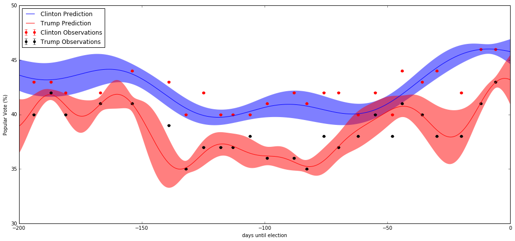
Although it’s predicting a Clinton victory in the popular vote, it seems remarkably close and the 95% confidence intervals have some overlap at the time of the election. For any given time-point we have a normal distribution for each prediction and we can then use this to calculate the probability of Clinton winning over Trump or vice versa. Of course in reality many other sources of data contribute towards a prediction. Gaussian processes, however provide a lot of flexibility for these types of data and importantly, can quantify the uncertainty of the prediction.