Introduction to Keras
Introduction
Keras is a high-level neural networks API, written in Python and capable of running on top of either TensorFlow or Theano. It was developed with a focus on enabling fast experimentation. Being able to go from idea to result with the least possible delay is key to doing good research.
If you’ve used scikit-learn then you should be on familiar ground as the library was developed with a similar philosophy.
- Can use either theano or tensorflow as a back-end. For the most part, you just need to set it up and then interact with it using keras. Ordering of dimensions can be different though.
- Models can be instantiated using the
Sequential()class. - Neural networks are built up from bottom layer to top using the
add()method. - Lots of recipes to follow and many examples for problems in natural language processing and image classification.
Before we start you can download the python notebook for this tutorial at https://github.com/sempwn/keras-intro
To begin we’ll make sure tensorflow and keras are installed. Open a terminal and type the following commands:
pip install --user tensorflow
pip install --user keras
The back-end of keras can either use theano or tensorflow. Verify that keras will use tensorflow by using the following command:
sed -i 's/theano/tensorflow/g' $HOME/.keras/keras.json
The keras library is very flexible, constantly being updated and being further integrated with tensorflow.
Another advantage is its intergration with tensorboard: A visualisation tool for neural network learning and debugging. If you’ve installed tensorflow already then you should already have it (check with: which tensorboard). Otherwise, run the command:
pip install tensorflow
We begin by importing the keras library as well as the Sequential model class which forms the basic skeleton
for our neural network. We’ll only consider one type of layer, where all the neurons in the layer are connected to all
the other neurons in the previous layer
import keras
from keras.models import Sequential
from keras.layers import Dense
Create the data
Let’s create some fake data. We’ll use the sci-kit learn library in order to do this.
%pylab inline
from sklearn.datasets import make_moons
from sklearn.preprocessing import scale
from sklearn.model_selection import train_test_split
X, Y = make_moons(noise=0.2, random_state=0, n_samples=1000)
X = scale(X)
X_train, X_test, Y_train, Y_test = train_test_split(X, Y, test_size=.5)
fig, ax = plt.subplots()
ax.scatter(X[Y==0, 0], X[Y==0, 1], label='Class 0')
ax.scatter(X[Y==1, 0], X[Y==1, 1], color='r', label='Class 1')
ax.legend()
ax.set(xlabel='X', ylabel='Y', title='Toy binary classification data set');
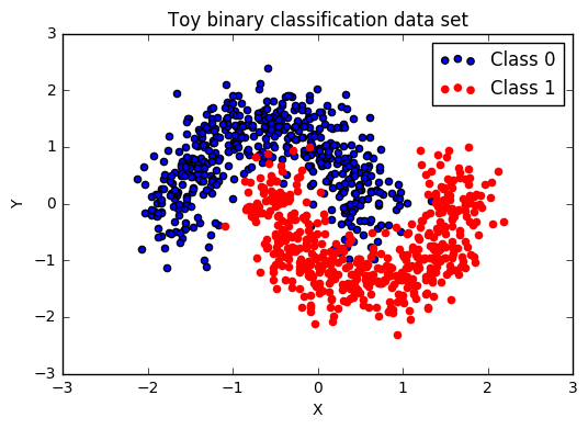
Our data has a binary class (0 or 1), with two input dimensions \(x\) and \(y\) and is visualized above. In order to correctly classify the data the neural network will need to successfully separate out the zig-zag shape that intersects where the two classes meet.
Creating the neural network
We’ll create a very simple multi-layer perceptron with one hidden layer.
This is done in keras by first defining a Sequential class object. Layers are then added from the initial layer,
which includes the data, hence we need to specify the number of input dimensions using the keyword input_dim. We also define the activation of this layer to be a rectified linear unit or relu.
Finally a densely connected layer is added with one output and a sigmoid activation corresponding to the binary class.
To fit this model we need to compile it by giving it the optimizer, loss and any additional metrics we want to consider in the training and validation.
#Create sequential  multi-layer perceptron
#uncomment if you want to add more layers (in the interest of time we use a shallower model)
model = Sequential()
model.add(Dense(32, input_dim=2,activation='relu')) #X,Y input dimensions. connecting to 32 neurons with relu activation
model.add(Dense(1, activation='sigmoid')) #binary classification so one output

model.compile(optimizer='AdaDelta',
              loss='binary_crossentropy',
              metrics=['accuracy'])
Adding in a callback for tensorboard
Next we define a callback for the model. This basically tells keras what format and where to write the data such that tensorboard can read it. Using the sub-folder structure as below allows us to compare between multiple models or multiple optimizations of the same model.
tb_callback = keras.callbacks.TensorBoard(log_dir='./Graph/model_1/',
                                          histogram_freq=0, write_graph=True,
                                          write_images=False)
Now perform the model fitting. Note where we’ve added in the callback.
model.fit(X_train, Y_train, batch_size=32, epochs=200,
          verbose=0, validation_data=(X_test, Y_test),callbacks=[tb_callback])
score = model.evaluate(X_test, Y_test, verbose=0)
print('Test loss:', score[0])
print('Test accuracy:', score[1])
('Test loss:', 0.15703605085611344)
('Test accuracy:', 0.93799999999999994)
93% isn’t bad. Running for a shorter number of epochs produces a lower accuracy, but running for a longer number of epochs may result in overfitting. It’s always worth comparing how the validation and training accuracy change at the end of each epoch.
Plotting the model prediction across the grid
We can create a grid of \((x,y)\) values and then predict the class probability on each of these values using our fitted model. We’ll then plot the original data with the underlying probabilities to see what the classification looks like and how it compares to the data
grid = np.mgrid[-3:3:100j,-3:3:100j]
grid_2d = grid.reshape(2, -1).T
X, Y = grid
prediction_probs = model.predict_proba(grid_2d, batch_size=32, verbose=0)
##plot results
fig, ax = plt.subplots(figsize=(10, 6))
contour = ax.contourf(X, Y, prediction_probs.reshape(100, 100))
ax.scatter(X_test[Y_test==0, 0], X_test[Y_test==0, 1])
ax.scatter(X_test[Y_test==1, 0], X_test[Y_test==1, 1], color='r')
cbar = plt.colorbar(contour, ax=ax)
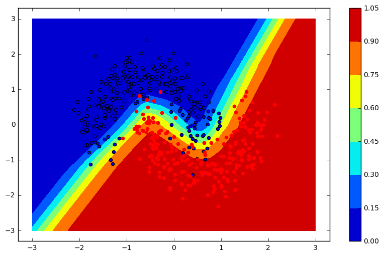
As you can see in the graph above, the model able to fully capture the zig-zag pattern needed to fully separate the classes. We could experiment by adding more layers or additional input ( \(xy\) for instance).
Visualising results
Now we visualize the results by running the following in the same terminal as this script
tensorboard --logdir $(pwd)/Graph
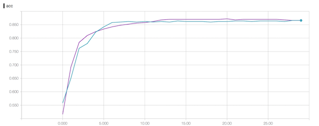
This runs a local server where we can view the results in browser. The plot below gives an example of what can be visualized. Here we ran the same model for the same number of epochs (remember to specify a new subfolder for each instance in order to compare the results). Tensorboard has many more features including visualization of the neural network. You can check out the documentation here
Conclusion
This was a trivial example of the use of keras on some test data. The real power comes when we start to consider convolutional or recurrent neural networks. More on this soon.