Introduction to convolutional neural networks

Preamble

Python notebook for this post can be found at https://github.com/sempwn/keras-intro

Before starting we’ll need to make sure tensorflow and keras are installed. Open a terminal and type the following commands:

pip install --user tensorflow
pip install --user keras --upgrade

The back-end of keras can either use theano or tensorflow. Verify that keras will use tensorflow by using the following command:

sed -i 's/theano/tensorflow/g' $HOME/.keras/keras.json

Note that this post was written in keras 2.0, where there have been a number of changes from version 1.0. We begin by loading in the libraries we’ll be using in the notebook

%pylab inline
import keras
from keras.datasets import mnist
from keras.models import Sequential
from keras.layers import Dense, Dropout, Activation, Flatten
from keras.layers import Conv2D, MaxPooling2D
from keras.utils import np_utils
from keras import backend as K

Populating the interactive namespace from numpy and matplotlib

Convolutional neural networks : A very brief introduction

To quote wikipedia:

Convolutional neural networks are biologically inspired variants of multilayer perceptrons, designed to emulate the behaviour of a visual cortex. These models mitigate the challenges posed by the MLP architecture by exploiting the strong spatially local correlation present in natural images.

One principle in machine learning is to create a feature map for data and then use your favourite classifier on those features. For image data this might be presence of straight lines, curved lines, placement of holes etc. This strategy can be very problem dependent. Instead of having to feature engineer for each specific problem, it would be better to automatically generate the features and combine with the classifier. CNNs are a way to achieve this.

Automatic feature engineering

Filters or convolution kernels can be treated like automatic feature detectors. A number of filters can be set before hand. For each filter, a convolution with this and part of the input is done for each part of the image. Weights for each filter are shared to reduce location dependency and reduce the number of parameters. The end result is a multi-dimensional matrix of copies of the original data with each filter applied to it.

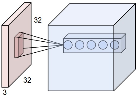
For a classification task, after one or more convolutional layers a number of fully connected layers can be added. The final layer has the same output as the number of classes.

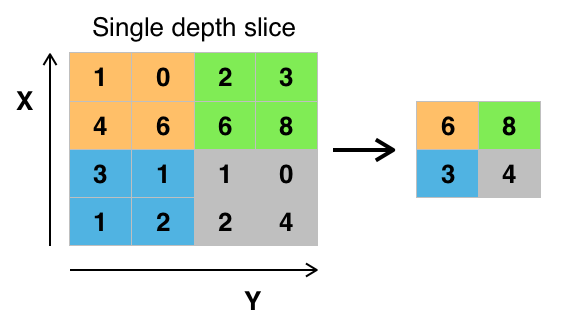
Pooling

Once convolutions have been performed across the whole image, we need someway of down-sampling. The easiest and most common way is to perform max pooling. For a certain pool size return the maximum from the filtered image of that subset is given as the output. A diagram of this is shown below

MNIST data set

We’ll begin by loading in the MNIST data set, which is a standard set of 28x28 grayscale images of handwritten numerical digits. Keras comes with it built in and automatically splits the data into a training and validation set.

# the data, shuffled and split between train and test sets
(x_train, y_train), (x_test, y_test) = mnist.load_data()

Convolutions on image

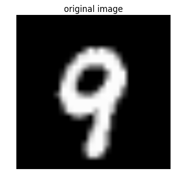
Let’s get some insight into what a random filter applied to a test image does. We’ll compare this to the trained filters at the end.

Each filtered pixel in the image is defined by \(C_i = \sum_j{I_{i+j-k} W_j}\), where \(W\) is the filter (sometimes known as a kernel), \(j\) is the 2D spatial index over \(W\), \(I\) is the input and \(k\) is the coordinate of the center of \(W\), specified by origin in the input parameters.

from scipy import signal
i = np.random.randint(x_train.shape[0])



c = x_train[i,:,:]
plt.imshow(c,cmap='gray'); plt.axis('off');
plt.title('original image');
plt.figure(figsize=(18,8))
for i in range(10):
    k = -1.0 + 1.0*np.random.rand(3,3)
    c_digit = signal.convolve2d(c, k, boundary='symm', mode='same');
    plt.subplot(2,5,i+1);
    plt.imshow(c_digit,cmap='gray'); plt.axis('off');

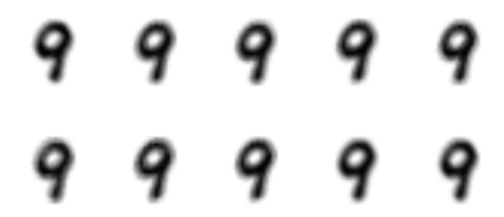
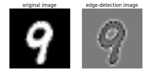
As you can see the random filters aren’t capable of differentiating different parts or features of the image. We do know however that non-random filters are very good at things like edge detection. Let’s compare these random filters above to a standard edge-detection filter. One such filter is used below

#define edge-detection filter
k = [
    [0, 1, 0],
    [1,-4, 1],
    [0, 1, 0]
    ]

plt.figure();
plt.subplot(1,2,1);
plt.imshow(c,cmap='gray'); plt.axis('off');
plt.title('original image');

plt.subplot(1,2,2);
c_digit = signal.convolve2d(c, k, boundary='symm', mode='same');
plt.imshow(c_digit,cmap='gray'); plt.axis('off');
plt.title('edge-detection image');   

Keras introduction

We’re using keras to construct and fit the convolutional neural network. Quoting their website

Keras is a high-level neural networks API, written in Python and capable of running on top of either TensorFlow or Theano. It was developed with a focus on enabling fast experimentation. Being able to go from idea to result with the least possible delay is key to doing good research.

We can rapidly develop a convolutional neural network in order to experiment with our image classification task. The first step will be to pre-process the data into a form that can be fed into a keras model

batch_size = 128
nb_classes = 10
nb_epoch = 6

# input image dimensions
img_rows, img_cols = 28, 28
# number of convolutional filters to use
nb_filters = 32
# size of pooling area for max pooling
pool_size = (2, 2)
# convolution kernel size
kernel_size = (3, 3)

if K.image_data_format() == 'channels_first':
    x_train = x_train.reshape(x_train.shape[0], 1, img_rows, img_cols)
    x_test = x_test.reshape(x_test.shape[0], 1, img_rows, img_cols)
    input_shape = (1, img_rows, img_cols)
else:
    x_train = x_train.reshape(x_train.shape[0], img_rows, img_cols, 1)
    x_test = x_test.reshape(x_test.shape[0], img_rows, img_cols, 1)
    input_shape = (img_rows, img_cols, 1)

#sub-sample of test data to improve training speed. Comment out
#if you want to train on full dataset.
x_train = x_train[:20000,:,:,:]
y_train = y_train[:20000]

#normalise the images and double check the shape and size of the image data
x_train = x_train.astype('float32')
x_test = x_test.astype('float32')
x_train /= 255
x_test /= 255
print('x_train shape:', x_train.shape)
print(x_train.shape[0], 'train samples')
print(x_test.shape[0], 'test samples')

# convert class vectors to binary class matrices
y_test_inds = y_test.copy()
y_train_inds = y_train.copy()
y_train = keras.utils.to_categorical(y_train, nb_classes)
y_test = keras.utils.to_categorical(y_test, nb_classes)

('x_train shape:', (20000, 28, 28, 1))
(20000, 'train samples')
(10000, 'test samples')

Tricks to avoid overfitting

20000 data-points isn’t a huge amount for the size of the models we’re considering.

• One trick to avoid overfitting is to use drop-out. This is where a weight is randomly assigned zero with a given probability to avoid the model becoming too dependent on a small number of weights.
• We can also consider ridge or LASSO regularisation as a way of trimming down the dependency and effective number of parameters.
• Early stopping and Batch Normalisation are other strategies to help control over-fitting.

Constructing the model

The model we’ll be using for classification will be a simple one convolutional layer plus one fully connected layer convolutional neural network. This is probably the simplest convolutional neural network that could be constructed so it’ll be interesting to see how it performs. We also introduce dropout between the two layers as our preferred method of avoiding overfitting.

#Create sequential convolutional multi-layer perceptron with max pooling and dropout
#uncomment layers below to produce a more accurate score (in the interest of time we use a shallower model)
model = Sequential()
model.add(Conv2D(nb_filters, kernel_size=(3, 3),
                 activation='relu',
                 input_shape=input_shape))  
#model.add(Conv2D(64, (3, 3), activation='relu'))
model.add(MaxPooling2D(pool_size=(2, 2)))
model.add(Dropout(0.25))
model.add(Flatten())
#model.add(Dense(128, activation='relu'))
model.add(Dropout(0.5))
model.add(Dense(nb_classes, activation='softmax'))

model.compile(loss=keras.losses.categorical_crossentropy,
              optimizer=keras.optimizers.Adam(),
              metrics=['accuracy'])

let’s see what we’ve constructed layer by layer. This is useful for checking the shapes of each layer are what you expect. Note that in the first layer the images are now 26x26. This is due to the convolution avoiding going over the edge of the image and so chopping off the outer border of the image.

model.summary()

_________________________________________________________________
Layer (type)                 Output Shape              Param #   
=================================================================
conv2d_1 (Conv2D)            (None, 26, 26, 32)        320       
_________________________________________________________________
max_pooling2d_1 (MaxPooling2 (None, 13, 13, 32)        0         
_________________________________________________________________
dropout_1 (Dropout)          (None, 13, 13, 32)        0         
_________________________________________________________________
flatten_1 (Flatten)          (None, 5408)              0         
_________________________________________________________________
dropout_2 (Dropout)          (None, 5408)              0         
_________________________________________________________________
dense_1 (Dense)              (None, 10)                54090     
=================================================================
Total params: 54,410.0
Trainable params: 54,410.0
Non-trainable params: 0.0
_________________________________________________________________

Model fitting

We can now fit the model to the data. We provide the batch size, number of epochs as well as the validation data. We also want the output to be verbose so we’re able to see how the log-loss and accuracy in both the test and validation set changes at the end of each epoch.

model.fit(x_train, y_train, batch_size=batch_size, epochs=nb_epoch,
          verbose=1, validation_data=(x_test, y_test))
score = model.evaluate(x_test, y_test, verbose=0)
print('Test loss:', score[0])
print('Test accuracy:', score[1])

Train on 20000 samples, validate on 10000 samples
Epoch 1/6
20000/20000 [==============================] - 16s - loss: 0.7113 - acc: 0.8046 - val_loss: 0.2958 - val_acc: 0.9171
Epoch 2/6
20000/20000 [==============================] - 15s - loss: 0.3009 - acc: 0.9114 - val_loss: 0.2093 - val_acc: 0.9425
Epoch 3/6
20000/20000 [==============================] - 15s - loss: 0.2325 - acc: 0.9317 - val_loss: 0.1689 - val_acc: 0.9548
Epoch 4/6
20000/20000 [==============================] - 16s - loss: 0.1853 - acc: 0.9460 - val_loss: 0.1385 - val_acc: 0.9620
Epoch 5/6
20000/20000 [==============================] - 15s - loss: 0.1610 - acc: 0.9524 - val_loss: 0.1216 - val_acc: 0.9660
Epoch 6/6
20000/20000 [==============================] - 15s - loss: 0.1451 - acc: 0.9571 - val_loss: 0.1103 - val_acc: 0.9685
('Test loss:', 0.11029711169451475)
('Test accuracy:', 0.96850000000000003)

Results

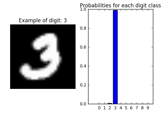
Let’s take a random digit example to find out how confident the model is at classifying the correct category

#choose a random data from test set and show probabilities for each class.
i = np.random.randint(0,len(x_test))
digit = x_test[i].reshape(28,28)

plt.figure();
plt.subplot(1,2,1);
plt.title('Example of digit: {}'.format(y_test_inds[i]));
plt.imshow(digit,cmap='gray'); plt.axis('off');
probs = model.predict_proba(digit.reshape(1,28,28,1),batch_size=1)
plt.subplot(1,2,2);
plt.title('Probabilities for each digit class');
plt.bar(np.arange(10),probs.reshape(10),align='center'); plt.xticks(np.arange(10),np.arange(10).astype(str));

1/1 [==============================] - 0s

Wrong predictions

Let’s look more closely at the predictions on the test data that weren’t correct

predictions = model.predict_classes(x_test, batch_size=32, verbose=1)

 9792/10000 [============================>.] - ETA: 0s

inds = np.arange(len(predictions))
wrong_results = inds[y_test_inds!=predictions]

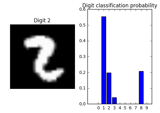
Example of an incorrectly labelled digit

We’ll choose randomly from the test set a digit that was incorrectly labelled and then plot the probabilities predicted for each class. We find that for an incorrectly labelled digit, the probabilities are in general lower and more spread between classes than for a correctly labelled digit.

#choose a random wrong result from the test set
i = np.random.randint(0,len(wrong_results))
i = wrong_results[i]
digit = x_test[i].reshape(28,28)

plt.figure();

plt.subplot(1,2,1);
plt.title('Digit {}'.format(y_test_inds[i]));
plt.imshow(digit,cmap='gray'); plt.axis('off');
probs = model.predict_proba(digit.reshape(1,28,28,1),batch_size=1)
plt.subplot(1,2,2);
plt.title('Digit classification probability');
plt.bar(np.arange(10),probs.reshape(10),align='center'); plt.xticks(np.arange(10),np.arange(10).astype(str));

1/1 [==============================] - 0s

Comparison between incorrectly labelled digits and all digits

It seems like for the example digit the prediction is a lot less confident when it’s wrong. Is this always the case? Let’s look at this by examining the maximum probability in any category for all digits that are incorrectly labelled.

prediction_probs = model.predict_proba(x_test, batch_size=32, verbose=1)

 9856/10000 [============================>.] - ETA: 0s

wrong_probs = np.array([prediction_probs[ind][digit] for ind,digit in zip(wrong_results,predictions[wrong_results])])
all_probs =  np.array([prediction_probs[ind][digit] for ind,digit in zip(np.arange(len(predictions)),predictions)])
#plot as histogram
plt.hist(wrong_probs,alpha=0.5,normed=True,label='wrongly-labeled');
plt.hist(all_probs,alpha=0.5,normed=True,label='all labels');
plt.legend();
plt.title('Comparison between wrong and correctly classified labels');
plt.xlabel('highest probability');

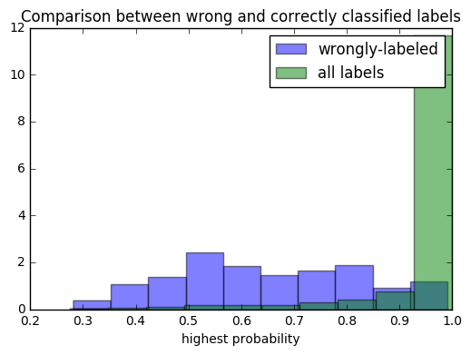
It appears in general that when a digit is wrongly labelled, the model provides it with a lower probability than when it’s correctly labelled. We would expect these two groups to become more separate as the model accuracy increases.

What’s been fitted ?

Let’s look at the convolutional layer of the model and the kernels that have been learnt. First we’ll check the dimensions of the first layer to see what we need to extract.

print (model.layers[0].get_weights()[0].shape)

(3, 3, 1, 32)

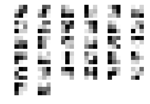
Now let’s visualise the learnt filters. Remember each of these filters are convolved with the image in order to produce a set of filtered images that can be used for classification.

weights = model.layers[0].get_weights()[0]
for i in range(nb_filters):
    plt.subplot(6,6,i+1)
    plt.imshow(weights[:,:,0,i],cmap='gray',interpolation='none'); plt.axis('off');

Visualising intermediate layers in the CNN

In order to visualise the activations half-way through the CNN and have some sense of what these convolutional kernels do to the input we need to create a new model with the same structure as before, but with the final layers missing. We then give it the weights it had previously and then predict on a given input. We now have a model that provides as output the convolved input passed through the activation for each of the learnt filters (32 all together).

#Create new sequential model, same as before but just keep the convolutional layer.
model_new = Sequential()
model_new.add(Conv2D(nb_filters, kernel_size=(3, 3),
                 activation='relu',
                 input_shape=input_shape))

#set weights for new model from weights trained on MNIST.
for i in range(1):
    model_new.layers[i].set_weights(model.layers[i].get_weights())

#pick a random digit and "predict" on this digit (output will be first layer of CNN)
i = np.random.randint(0,len(x_test))
digit = x_test[i].reshape(1,28,28,1)
pred = model_new.predict(digit)

#check shape of prediction
print pred.shape

(1, 26, 26, 32)

#For all the filters, plot the output of the input
plt.figure(figsize=(18,18))
filts = pred[0]
for i in range(nb_filters):
    filter_digit = filts[:,:,i]
    plt.subplot(6,6,i+1)
    plt.imshow(filter_digit,cmap='gray'); plt.axis('off');

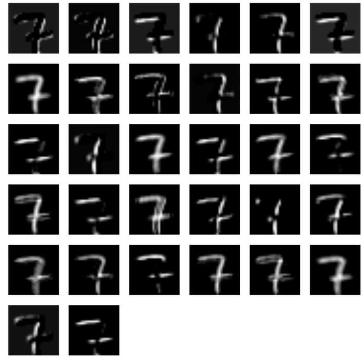
The filters pick out a lot of details from the image including horizontal and vertical lines as well as edges and potentially the terminal points of lines. We’ve only created one convolutional layer in our model. The real power comes when these convolutional layers are stacked together, creating a mechanism by which more general filters can be learnt.