Probabilistic programming 3: Bayesian probability

Introduction

This is part three in a series on probabilistic programming. Part one introduces Monte Carlo simulation and part two introduces the concept of the Markov chain. In this post I’ll introduce the concept of Bayes rule, which is the main machinery at the heart of Bayesian inference.

The diagram above represents a probability of two events: A and B. A could be testing positive for an infection and B could be actually have the infection. These events are clearly not independent and so we need some way of establishing their relationship as the probability of observing one is dependent on observing the other. How can we quantify this? One way is to look at the intersection of both events or in set notation $A \cap B$. We call the corresponding probability of both events happening $P(A,B)$. What if we already know that an event has occurred? Say we know event $A$ already, what would the probability of $B$ be given we know $A$ is true? Looking at the above diagram we see this would be the area of the intersection divided by the total area of $A$. We can represent this formula as $P(B | A) = P(A,B)/P(A)$. Which can be read as “The probability of B given A is the probability of A and B divided by the probability of A”.

What if we now wanted to know what the probability of A is given B? Well, we can just swap the symbols around in the previous formula to get $P(A | B) = P(A,B)/P(B)$. You’ll notice that we can now define the probability of A and B based on conditional probabilities, $P(A|B)P(B)$ or $P(B|A)P(A)$. If we equate these two and re-arrange we get the following:

\(P(A|B) = \frac{P(B|A)P(A)}{P(B)}\)

This is known as Bayes’ rule and is the entire basis of Bayesian statistics. Its power comes in the ability to take the probability of A on B and invert the relationship to give the probability of B given A.

Sensitivity and specificity

One application of this rule is in DNA or disease testing. We can discover the probability of testing positive given that an individual actually has the disease through repeated measurements of a given test. However, what we’d really want to know is whether someone actually has a disease given that they tested positive. Test accuracy can be described in terms of their sensitivity and specificity. Sensitivity is the probability of testing positive given a positive case and specificity is the probability of testing negative given a negative case. We can invert this relationship using Bayes rule:

\(P(+ve | +ve test) = \frac{P(\text{+ve test} | \text{+ve}) P(\text{+ve})}{P(\text{+ve test})}.\)

There’s a trick here where we can define the probability of a positive test by considering all the associated conditional probabilities (known as the law of total probability),

\(P(\text{+ve test}) = P(\text{+ve test} | \text{+ve})P(\text{+ve}) + P(\text{+ve test} | \text{-ve})P(\text{-ve}).\)

So it turns out in order to find the probability of being positive given a positive test we need to know what the underlying probability of actually being positive is (known as the base rate). We can see what the consequences of this are in the interactive diagram below where we imagine that 1000 people have been tested and we also know their disease status. Try playing with the base rate, sensitivity and specificity.

If the base rate is low (1%), then even with a 99% sensitivity and specificity the probability of actually being positive if you tested positive is approximately 50%. This is an example of the prosecutor’s fallacy and shows how important it is to consider the base rate is of what you’re testing for.

This type of reasoning can be applied to a diverse set of problems. If you know the probability that someone has a certain gene given they have developed cancer, what is the probability that someone will develop cancer given they have that gene. In a spam filter you can calculate the probability that an email is spam if it contains a set of keywords in terms of the probability of an email containing certain keywords given it’s spam.

Causal belief

We don’t have to stop with one event dependent on another. We could also consider the impact of multiple events on one another in terms of their probabilities. This generalization is called Bayesian network theory.

Let’s consider the example where we’re deciding whether to take an umbrella with us or not based on the weather forecast. Causally, this looks like the following diagram:

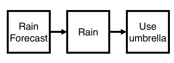
Here we’re modelling the conditional dependencies of three events: whether rain is forecast, whether it’s actually raining and whether you end up using an umbrella. Bayes rule gives us a way of inverting this dependency, by for example considering the probability of using an umbrella given rain was forecast. If A = rain forecast, B = raining and C = using an umbrella then the joint probability (the probability of all three events occurring) can be written as

\(P(A,B,C) = P(A)P(B|A)P(C|B)\)

You can see how changes in these probabilities impacts the conditional dependencies in the tool below.

This may seem like a slightly trivial example, but this type of model has a huge amount of application. See for example, Latent Dirichlet Allocation in natural language processing, Bayesian Hierarchical Models or Restricted Boltzmann Machines.

Inference

One of the biggest applications of Bayes rule is in Bayesian inference. This is where we have some data $D$ (ex. No. of heads in 100 coin flips. or heights of individuals in a population) and a model parameterised by a set of parameters $\theta$ (e.g. probability of heads for a certain coin or mean and variance of population height) and we wish to calculate the probability $P(\theta|D)$. That is the probability of a certain set of parameters given the data we have observed (e.g. probability coin produces heads is 50% given we’ve observed 100 coin flips that produced 75 heads). Applying Bayes rule, we see that

\(P(\theta | D) = \frac{P(D | \theta) P(\theta)}{P(D)}\).

We can therefore write down our desired probability in terms of the probability of observing some data given some model parameters (known as the likelihood) and the probability of a given set of parameters (known as the prior). We also have a tricky Probability of observing the data $D$ to deal with- let’s ignore this for now.

What if we observed some new data $D_2$? Say we decided to flip the coin again 100 times or we get more data on a population. We can apply Bayes’ rule again in a similar fashion as before to produce,

\(P(\theta | D_2,D) = \frac{P(D_2 | \theta ) P(D | \theta) P(\theta)}{P(D) P(D_2)}\).

We can then update our posterior each time we observe new data.

This is all a bit abstract, let’s look at an actual example. Imagine we have discovered a new cure for a disease and we want to estimate its efficacy, but we only had a limited amount of data to date. We can assume each patient is independent of one another (is this reasonable? Could how a trial has been set-up change this?) and say that someone is cured with the treatment with a probability $p$. Each individual then has a probability of being cured $p$ and not being cured $1-p$. Now what if our trial had $N$ patients, what is the probability of seeing $x$ people cured? We can calculate this using the binomial distribution (this is just a distribution that counts up all the ways $x$ people can be cured out of $N$ people and sums up the probability for each event). We now have a likelihood, but we also need a prior in order to perform inference. There’s a trick where we can take a prior that has a special shape, so that we can write down the posterior analytically. This trick is called conjugate priors. For this example we can interpret the prior as having observed a previous trial where $y$ people were cured out of $M$ individuals.

The tool below allows us to explore the consequences of this. We can change how many patients were in the prior dataset and also in the current dataset as well as change how many individuals were cured or not (by clicking on them). Below that is a plot of the likelihood for the new dataset as well as the posterior representing the probability of the cure rate incorporating both datasets.

Prior

Data

Some interesting things spring out of this. First, in the limit of a small amount of data, even if all patients are cured we don’t spring to the conclusion that the cure rate is 100%. Similarly, if we have little new information then this doesn’t change our posterior beliefs all that much.

This works nicely for such a simple example, but what if patients came from different populations where we know the cure rate is different? This leads on to Bayesian Hierarchical Modelling, but makes the inference calculation a lot more involved.

The power of Bayesian probability comes from its ability to deal with combining new information with other information or beliefs and its ability to deal with small or missing data.

Acknowledgements

The code for the Venn diagram can be found here.

All the interactive examples were coded in d3, which has many fantastic examples for data visualization.