library(rstan)
#> Loading required package: StanHeaders
#>
#> rstan version 2.32.7 (Stan version 2.32.2)
#> For execution on a local, multicore CPU with excess RAM we recommend calling
#> options(mc.cores = parallel::detectCores()).
#> To avoid recompilation of unchanged Stan programs, we recommend calling
#> rstan_options(auto_write = TRUE)
#> For within-chain threading using `reduce_sum()` or `map_rect()` Stan functions,
#> change `threads_per_chain` option:
#> rstan_options(threads_per_chain = 1)
library(bennu)
library(bayesplot)
#> This is bayesplot version 1.14.0
#> - Online documentation and vignettes at mc-stan.org/bayesplot
#> - bayesplot theme set to bayesplot::theme_default()
#>    * Does _not_ affect other ggplot2 plots
#>    * See ?bayesplot_theme_set for details on theme setting
library(ggplot2)

rstan_options(auto_write = TRUE)
options(mc.cores = 2)

## basic example code
d <- generate_model_data()
#> Warning: `generate_model_data()` was deprecated in bennu 0.2.1.
#> ℹ Please use `model_random_walk_data()` instead.
#> This warning is displayed once every 8 hours.
#> Call `lifecycle::last_lifecycle_warnings()` to see where this warning was
#> generated.
# note iter should be at least 2000 to generate a reasonable posterior sample
fit <- est_naloxone(d, iter = 100)
#> ds (Total)
#> Chain 1:
#> Chain 2:
#> Chain 2:  Elapsed Time: 0.09 seconds (Warm-up)
#> Chain 2:                0.11 seconds (Sampling)
#> Chain 2:                0.2 seconds (Total)
#> Chain 2:
#> Warning: There were 7 divergent transitions after warmup. See
#> https://mc-stan.org/misc/warnings.html#divergent-transitions-after-warmup
#> to find out why this is a problem and how to eliminate them.
#> Warning: There were 1 chains where the estimated Bayesian Fraction of Missing Information was low. See
#> https://mc-stan.org/misc/warnings.html#bfmi-low
#> Warning: Examine the pairs() plot to diagnose sampling problems
#> Warning: The largest R-hat is NA, indicating chains have not mixed.
#> Running the chains for more iterations may help. See
#> https://mc-stan.org/misc/warnings.html#r-hat
#> Warning: Bulk Effective Samples Size (ESS) is too low, indicating posterior means and medians may be unreliable.
#> Running the chains for more iterations may help. See
#> https://mc-stan.org/misc/warnings.html#bulk-ess
#> Warning: Tail Effective Samples Size (ESS) is too low, indicating posterior variances and tail quantiles may be unreliable.
#> Running the chains for more iterations may help. See
#> https://mc-stan.org/misc/warnings.html#tail-ess
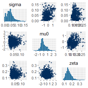
mcmc_pairs(fit,
  pars = c("sigma", "mu0", "zeta"),
  off_diag_args = list(size = 1, alpha = 0.5)
)
Return median and 90th percentiles for posterior samples
library(posterior)
#> This is posterior version 1.6.1
#>
#> Attaching package: 'posterior'
#> The following object is masked from 'package:bayesplot':
#>
#>     rhat
#> The following objects are masked from 'package:rstan':
#>
#>     ess_bulk, ess_tail
#> The following objects are masked from 'package:stats':
#>
#>     mad, sd, var
#> The following objects are masked from 'package:base':
#>
#>     %in%, match

summarise_draws(fit, default_summary_measures())
#> # A tibble: 222 × 7
#>    variable   mean median     sd    mad    q5   q95
#>    <chr>     <dbl>  <dbl>  <dbl>  <dbl> <dbl> <dbl>
#>  1 sim_p[1]  0.257  0.241 0.0827 0.0798 0.144 0.396
#>  2 sim_p[2]  0.261  0.256 0.0732 0.0745 0.154 0.403
#>  3 sim_p[3]  0.258  0.255 0.0601 0.0470 0.168 0.364
#>  4 sim_p[4]  0.243  0.240 0.0523 0.0473 0.165 0.335
#>  5 sim_p[5]  0.243  0.233 0.0590 0.0510 0.158 0.346
#>  6 sim_p[6]  0.242  0.234 0.0579 0.0484 0.158 0.338
#>  7 sim_p[7]  0.230  0.230 0.0416 0.0372 0.167 0.298
#>  8 sim_p[8]  0.242  0.241 0.0419 0.0388 0.168 0.309
#>  9 sim_p[9]  0.243  0.238 0.0464 0.0470 0.172 0.319
#> 10 sim_p[10] 0.252  0.248 0.0467 0.0414 0.186 0.336
#> # ℹ 212 more rows
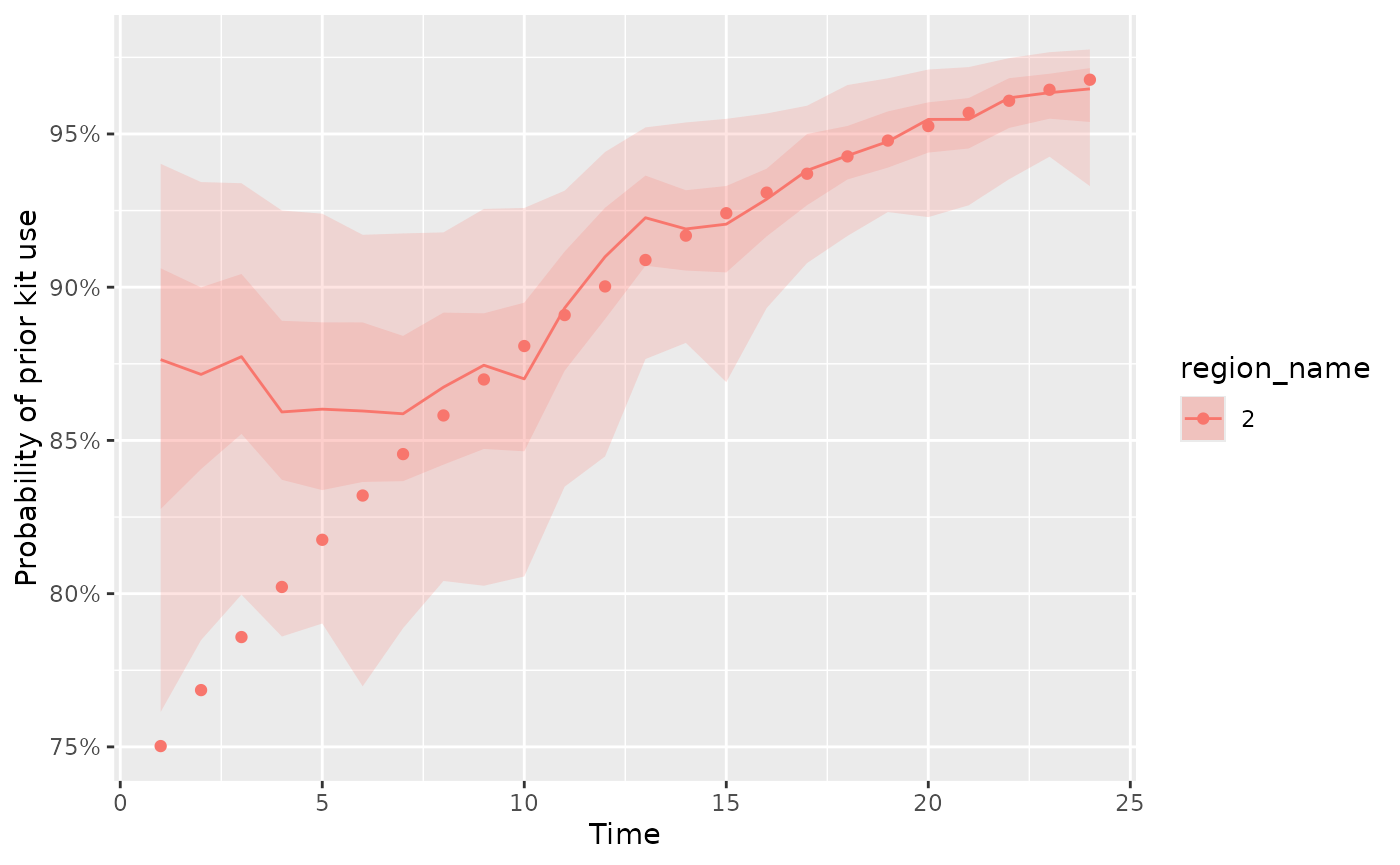
We can plot the posterior predictive distribution of the probability
of prior kit use and compare to simulated data using the
plot_kit_use function
plot_kit_use(model = fit, data = d)
We can also plot the reported number of kits used along with the
posterior predictive distribution using the plot_kit_use
function with the reported argument set to
TRUE
plot_kit_use(model = fit, reported = TRUE, data = d)
Alternatively, if we only want to plot certain regions we can include
that as an optional argument in the plot_kit_use
function
plot_kit_use(
  model = fit, data = d,
  regions_to_plot = c("2")
)
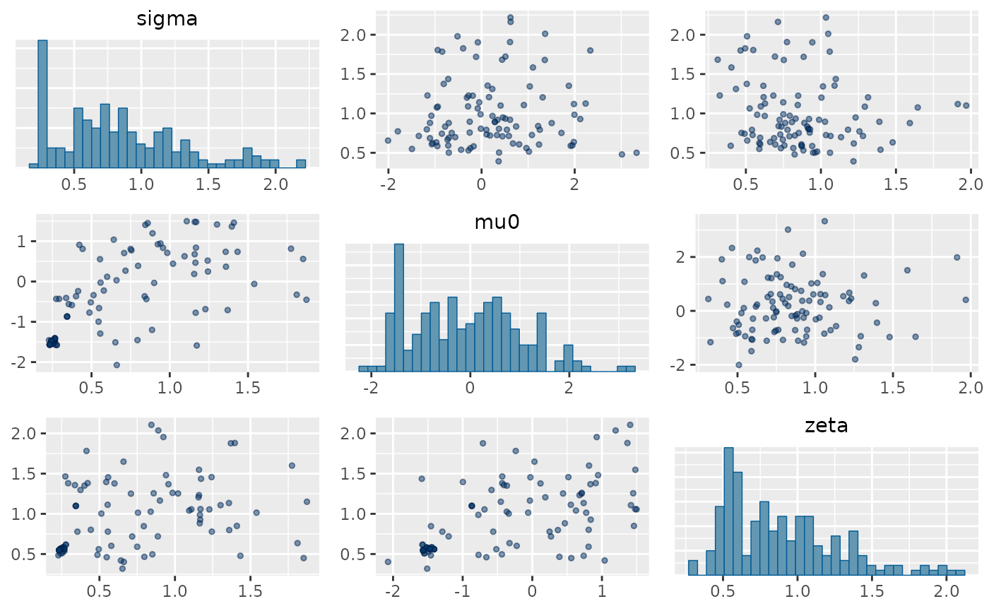
We can compare the posterior predictive check to the prior predictive
check by re-running the model without the likelihood by setting the
run_estimation parameter to FALSE
# note iter should be at least 2000 to generate a reasonable posterior sample
prior_fit <- est_naloxone(d,
  run_estimation = FALSE,
  iter = 100
)
#> 0 [100%]  (Sampling)
#> Chain 2:
#> Chain 2:  Elapsed Time: 0.108 seconds (Warm-up)
#> Chain 2:                0.099 seconds (Sampling)
#> Chain 2:                0.207 seconds (Total)
#> Chain 2:
#> Warning: There were 31 divergent transitions after warmup. See
#> https://mc-stan.org/misc/warnings.html#divergent-transitions-after-warmup
#> to find out why this is a problem and how to eliminate them.
#> Warning: There were 2 transitions after warmup that exceeded the maximum treedepth. Increase max_treedepth above 10. See
#> https://mc-stan.org/misc/warnings.html#maximum-treedepth-exceeded
#> Warning: There were 2 chains where the estimated Bayesian Fraction of Missing Information was low. See
#> https://mc-stan.org/misc/warnings.html#bfmi-low
#> Warning: Examine the pairs() plot to diagnose sampling problems
#> Warning: The largest R-hat is NA, indicating chains have not mixed.
#> Running the chains for more iterations may help. See
#> https://mc-stan.org/misc/warnings.html#r-hat
#> Warning: Bulk Effective Samples Size (ESS) is too low, indicating posterior means and medians may be unreliable.
#> Running the chains for more iterations may help. See
#> https://mc-stan.org/misc/warnings.html#bulk-ess
#> Warning: Tail Effective Samples Size (ESS) is too low, indicating posterior variances and tail quantiles may be unreliable.
#> Running the chains for more iterations may help. See
#> https://mc-stan.org/misc/warnings.html#tail-ess
mcmc_pairs(prior_fit,
  pars = c("sigma", "mu0", "zeta"),
  off_diag_args = list(size = 1, alpha = 0.5)
)
We can compare the prior and posterior predictive distribution of the
probability of prior kit use using the plot_kit_use
function
plot_kit_use(prior = prior_fit, posterior = fit, data = d)
Incorporating different priors
The default priors for the model are set to be weakly uninformative.
To change the default priors we can specify a list as
follows. Note that c is the prior of the region
coefficients, mu0 is the intercept, ct0 is the
initial conditions of the random walk, zeta is the standard
deviation of the random walk, and sigma is the standard
deviation of the error. In this example let’s set the variation month to
month to be smaller by setting the standard deviation of the prior for
zeta to 0.01.
nondefault_priors <- list(
  c = list(mu = 0, sigma = 1),
  ct0 = list(mu = 0, sigma = 1),
  zeta = list(mu = 0, sigma = 0.01),
  mu0 = list(mu = 0, sigma = 1),
  sigma = list(mu = 0, sigma = 1)
)
nondefault_prior_fit <- est_naloxone(d, iter = 100, priors = nondefault_priors)
#> [ 70%]  (Sampling)
#> Chain 1: Iteration: 80 / 100 [ 80%]  (Sampling)
#> Warning: There were 51 divergent transitions after warmup. See
#> https://mc-stan.org/misc/warnings.html#divergent-transitions-after-warmup
#> to find out why this is a problem and how to eliminate them.
#> Warning: There were 1 transitions after warmup that exceeded the maximum treedepth. Increase max_treedepth above 10. See
#> https://mc-stan.org/misc/warnings.html#maximum-treedepth-exceeded
#> Warning: Examine the pairs() plot to diagnose sampling problems
#> Warning: The largest R-hat is NA, indicating chains have not mixed.
#> Running the chains for more iterations may help. See
#> https://mc-stan.org/misc/warnings.html#r-hat
#> Warning: Bulk Effective Samples Size (ESS) is too low, indicating posterior means and medians may be unreliable.
#> Running the chains for more iterations may help. See
#> https://mc-stan.org/misc/warnings.html#bulk-ess
#> Warning: Tail Effective Samples Size (ESS) is too low, indicating posterior variances and tail quantiles may be unreliable.
#> Running the chains for more iterations may help. See
#> https://mc-stan.org/misc/warnings.html#tail-ess
Compare the posterior using non-default priors to the posterior for default priors,
plot_kit_use(`Default prior` = fit,
             `Non-default prior` = nondefault_prior_fit, data = d)
Random walk of order 2 model
The second model uses a random walk of order 1 to characterize the time-dependence structure of the inverse logit probability of naloxone use,
The model can also be fit using a random walk of order 2 increments for the inverse logit probability of naloxone use using the following independent second order increments,
This version of the model will produce smoother estimates of probability of naloxone use in time.
# note iter should be at least 2000 to generate a reasonable posterior sample
# note use `rw_type` to specify order of random walk
rw2_fit <- est_naloxone(d,
  rw_type = 2,
  iter = 100
)
#>  51%]  (Sampling)
#> Warning: There were 11 divergent transitions after warmup. See
#> https://mc-stan.org/misc/warnings.html#divergent-transitions-after-warmup
#> to find out why this is a problem and how to eliminate them.
#> Warning: There were 38 transitions after warmup that exceeded the maximum treedepth. Increase max_treedepth above 10. See
#> https://mc-stan.org/misc/warnings.html#maximum-treedepth-exceeded
#> Warning: Examine the pairs() plot to diagnose sampling problems
#> Warning: The largest R-hat is NA, indicating chains have not mixed.
#> Running the chains for more iterations may help. See
#> https://mc-stan.org/misc/warnings.html#r-hat
#> Warning: Bulk Effective Samples Size (ESS) is too low, indicating posterior means and medians may be unreliable.
#> Running the chains for more iterations may help. See
#> https://mc-stan.org/misc/warnings.html#bulk-ess
#> Warning: Tail Effective Samples Size (ESS) is too low, indicating posterior variances and tail quantiles may be unreliable.
#> Running the chains for more iterations may help. See
#> https://mc-stan.org/misc/warnings.html#tail-ess
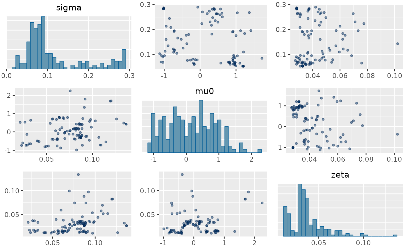
mcmc_pairs(rw2_fit,
  pars = c("sigma", "mu0", "zeta"),
  off_diag_args = list(size = 1, alpha = 0.5)
)
Summarize random walk order 2 model draws
summarise_draws(rw2_fit, default_convergence_measures())
#> # A tibble: 222 × 4
#>    variable   rhat ess_bulk ess_tail
#>    <chr>     <dbl>    <dbl>    <dbl>
#>  1 sim_p[1]   1.37     11.4     35.3
#>  2 sim_p[2]   1.42     10.2     84.9
#>  3 sim_p[3]   1.28     14.4    100.0
#>  4 sim_p[4]   1.30     12.7    103.
#>  5 sim_p[5]   1.10     34.2    134.
#>  6 sim_p[6]   1.10     66.2    121.
#>  7 sim_p[7]   1.10     85.0     72.1
#>  8 sim_p[8]   1.10     92.7    142.
#>  9 sim_p[9]   1.07     84.0     35.0
#> 10 sim_p[10]  1.07    141.     153.
#> # ℹ 212 more rows
We can compare two different model fits of the probability of prior
kit use to simulated data using the plot_kit_use
function
plot_kit_use(rw_1 = fit, rw_2 = rw2_fit, data = d)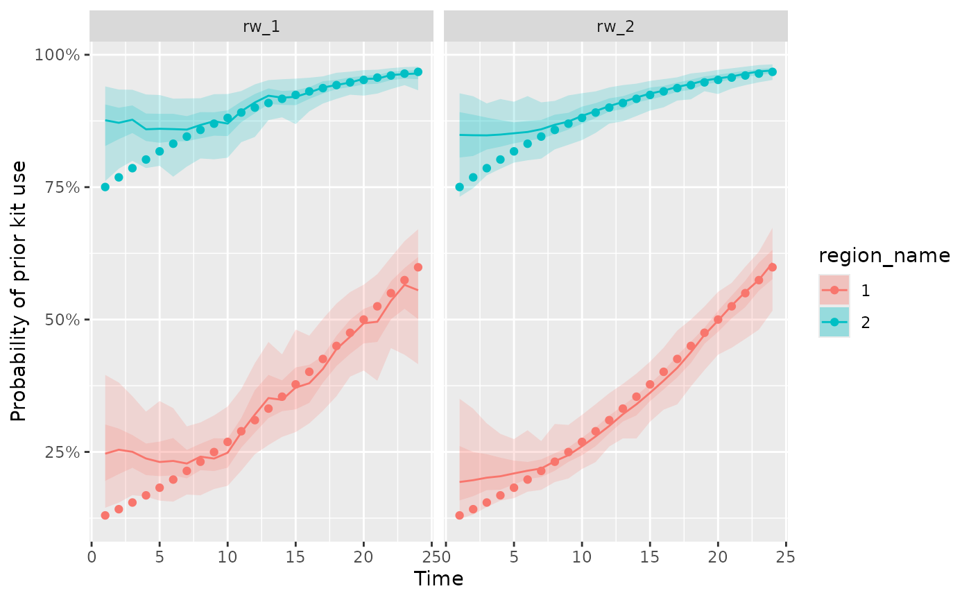
fit missing distribution data
As distribution data are reported from sites some months may not be reported. This would lead to a difference in the frequency of the orders data and the distribution data. The model can account for these differences and infer the distribution during missing months. See the following example for generating distribution data once every three months
## basic example code
d_missing <- generate_model_data(reporting_freq = 3)
ggplot(aes(x = times, y = Reported_Used, color = as.factor(regions)),
  data = d_missing
) +
  geom_point()
#> Warning: Removed 32 rows containing missing values or values outside the scale range
#> (`geom_point()`).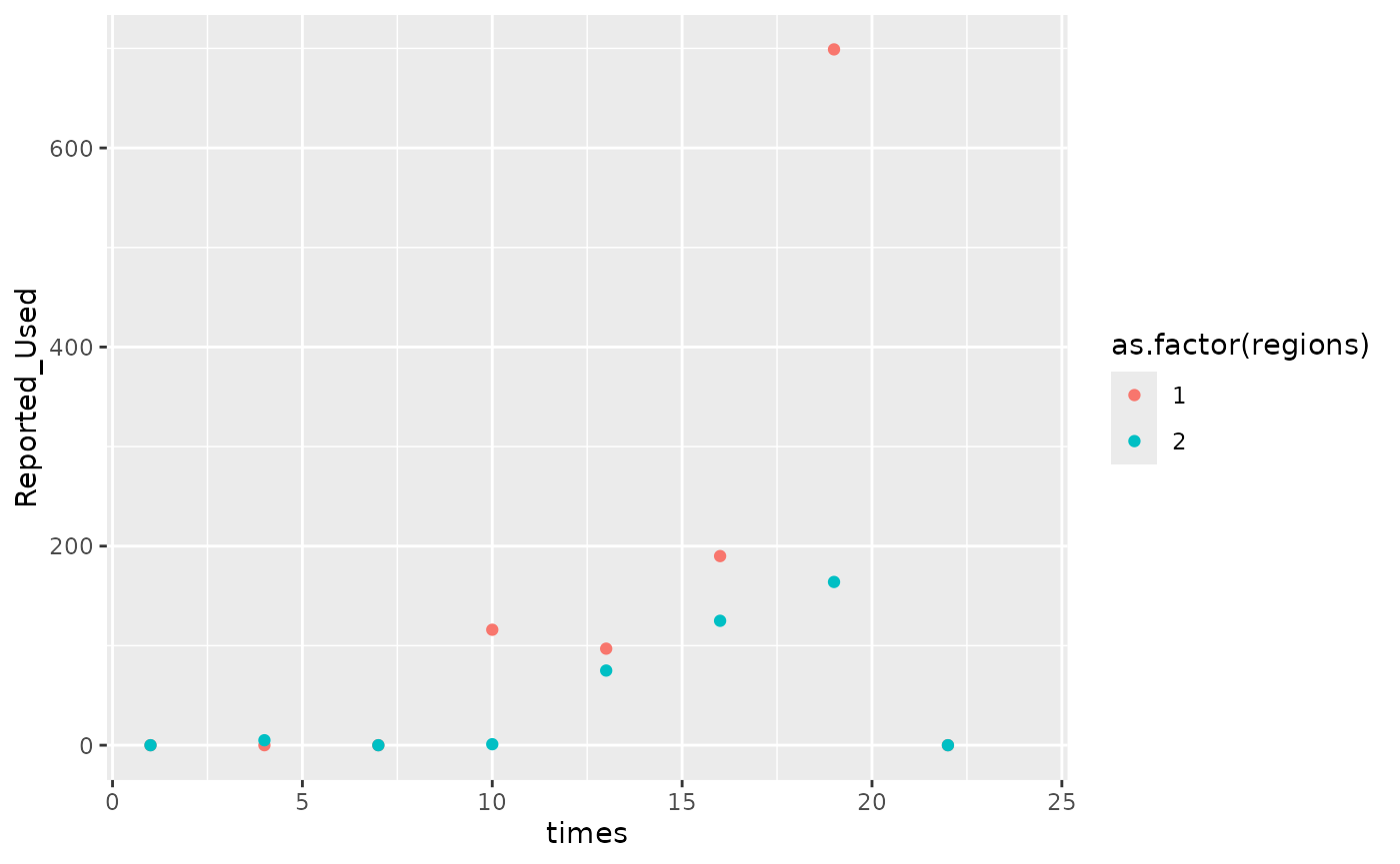
missing_fit <- est_naloxone(d_missing,
  rw_type = 2,
  iter = 100
)
#> 0 [100%]  (Sampling)
#> Chain 1:
#> Chain 1:  Elapsed Time: 0.132 seconds (Warm-up)
#> Chain 1:                0.126 seconds (Sampling)
#> Chain 1:                0.258 seconds (Total)
#> Chain 1:
#> Warning: There were 11 divergent transitions after warmup. See
#> https://mc-stan.org/misc/warnings.html#divergent-transitions-after-warmup
#> to find out why this is a problem and how to eliminate them.
#> Warning: There were 1 transitions after warmup that exceeded the maximum treedepth. Increase max_treedepth above 10. See
#> https://mc-stan.org/misc/warnings.html#maximum-treedepth-exceeded
#> Warning: Examine the pairs() plot to diagnose sampling problems
#> Warning: The largest R-hat is NA, indicating chains have not mixed.
#> Running the chains for more iterations may help. See
#> https://mc-stan.org/misc/warnings.html#r-hat
#> Warning: Bulk Effective Samples Size (ESS) is too low, indicating posterior means and medians may be unreliable.
#> Running the chains for more iterations may help. See
#> https://mc-stan.org/misc/warnings.html#bulk-ess
#> Warning: Tail Effective Samples Size (ESS) is too low, indicating posterior variances and tail quantiles may be unreliable.
#> Running the chains for more iterations may help. See
#> https://mc-stan.org/misc/warnings.html#tail-ess
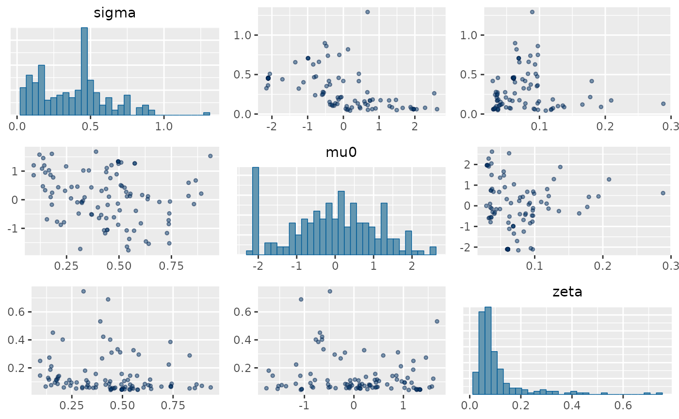
mcmc_pairs(missing_fit,
  pars = c("sigma", "mu0", "zeta"),
  off_diag_args = list(size = 1, alpha = 0.5)
)
plot_kit_use(model = missing_fit, data = d_missing)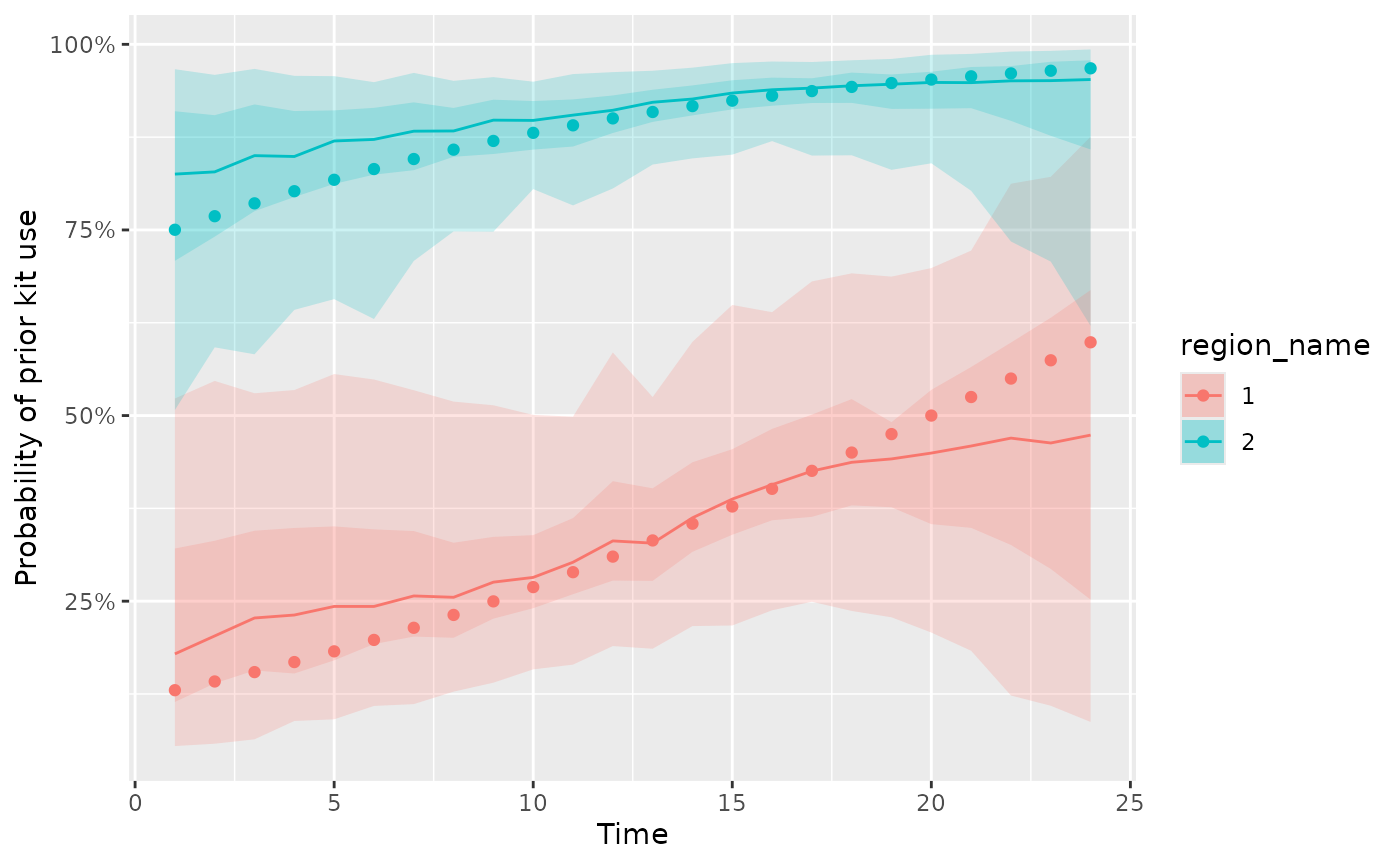
plot_kit_use(model = missing_fit, data = d_missing, reported = TRUE)
Change scale of data
the original model was designed for data aggregated into months. If the order and distribution data is aggregated differently then this can be incorporated into the model by updating the delay in reporting distribution and the delay in ordering to distributing distribution.
The delay in ordering to distributing distribution is composed of a gamma distribution with shape parameter and inverse scale parameter . In order to update for example from monthly to weekly data, we can use the following property of the gamma distribution,
To convert the delay distribution from month into week set as one over the approximate number of weeks in a month. The reporting delay distribution is a simple vector of length 3 denoting the empirical delay distribution. This can be expanded into months through interpolation and normalization to retain its property as a probability distribution. Example code (not run) is shown below. Note that these distributions will need to be updated when considering another jurisdiction,
# monthly reporting delay distribution
psi_vec <- c(0.7, 0.2, 0.1)
# convert to weeks using interpolation
weekly_psi_vec <- rep(psi_vec, 4) / sum(psi_vec)

# properties of order to distributed delay distribution in months
max_delays <- 3
delay_alpha <- 2
delay_beta <- 1

# convert to weeks
weekly_max_delays <- max_delays * 4
weekly_delay_alpha <- delay_alpha
weekly_delay_beta <- 0.25 * delay_beta

result <- est_naloxone(d,
  psi_vec = weekly_psi_vec,
  max_delays = weekly_max_delays,
  delay_alpha = weekly_delay_alpha,
  delay_beta = weekly_delay_beta
)