BC outbreak data fitting
Source:vignettes/BC_outbreak_data_fitting.Rmd
BC_outbreak_data_fitting.RmdLoad long-term healthcare outbreak data
Data loaded includes number of cases since outbreak on a given day for each location, the number of outbreaks, the size of the facility, as well as the labels for the outbreaks.
n_outbreaks <- length(BC_LTHC_outbreaks_100Imputs[[100]]$capacity)
outbreak_sizes <- BC_LTHC_outbreaks_100Imputs[[100]]$capacity
outbreak_cases_series <- BC_LTHC_outbreaks_100Imputs[[100]]$time_series
ob_codes <- BC_LTHC_outbreaks_100Imputs[[100]]$Location


outbreak_cases <- BC_LTHC_outbreaks_100Imputs[[100]]$case_matrix

tmax <- 64

# plot cases from matrix
as_tibble(outbreak_cases,rownames="time") %>%
  mutate(time = as.double(time)) %>%
  pivot_longer(-time,names_to = "location",values_to="cases") %>%
  ggplot(aes(x=time,y=cases,color=location)) +
  geom_line() +
  theme(legend.position = "none")
#> Warning: The `x` argument of `as_tibble.matrix()` must have unique column names if `.name_repair` is omitted as of tibble 2.0.0.
#> Using compatibility `.name_repair`.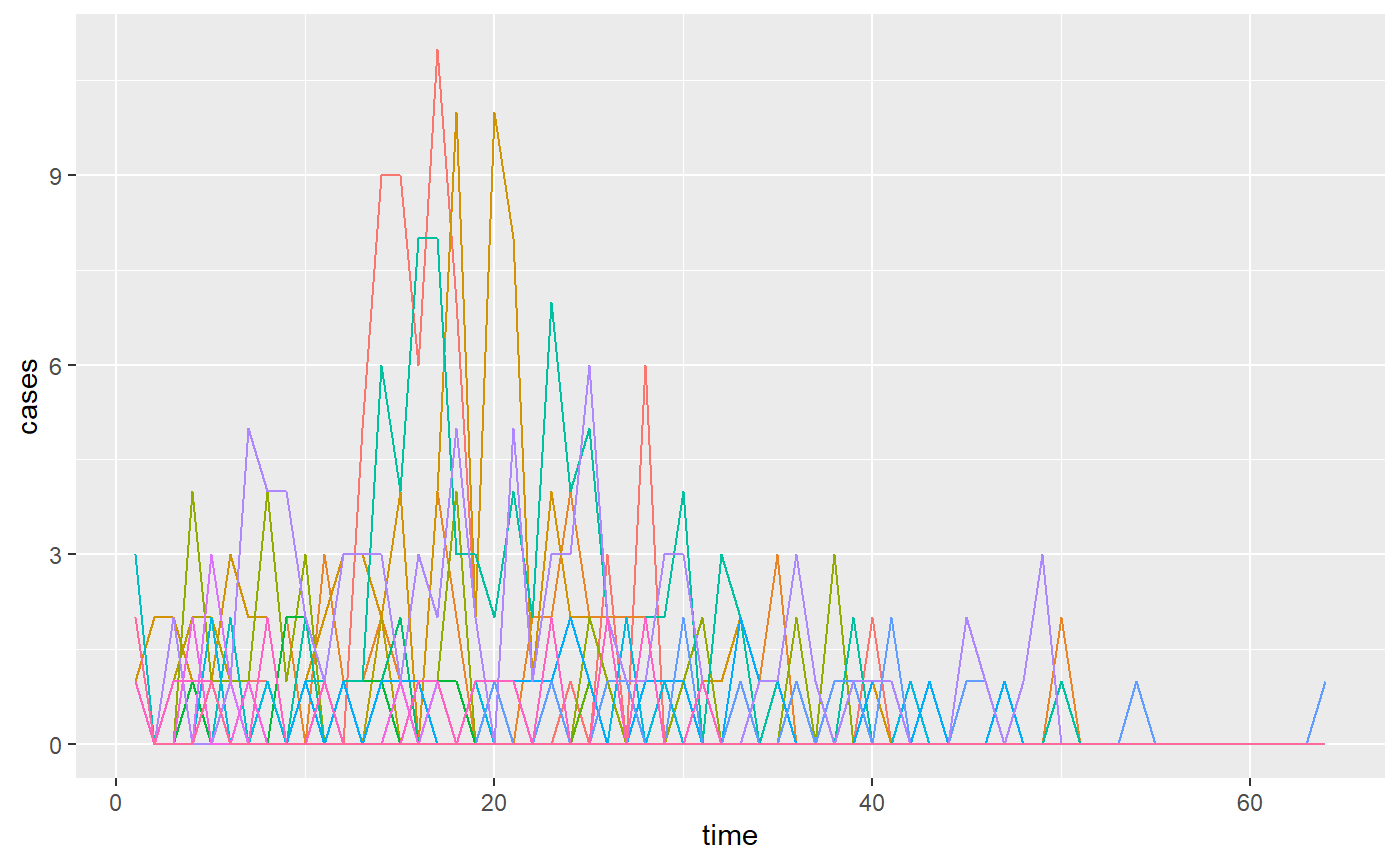
Fit model
Fit model including estimating intervention. This code chunk is not
run in the vignette, but provides the syntax for how to produce
posterior samples. The bc_fit data object is including in
the package.
stan_mod <- rstan::stan_model(system.file("stan", "hierarchical_SEIR_incidence_model.stan", package = "cr0eso"))

bc_fit <- seir_model_fit(
                       stan_model = stan_mod,
                       tmax,n_outbreaks,outbreak_cases,outbreak_sizes,
                       intervention_switch = TRUE,
                       multilevel_intervention = FALSE,
                       iter = 2000)
Model diagnostic checking
rstan::check_hmc_diagnostics(bc_fit$model)
#>
#> Divergences:
#> 0 of 4000 iterations ended with a divergence.
#>
#> Tree depth:
#> 0 of 4000 iterations saturated the maximum tree depth of 10.
#>
#> Energy:
#> E-BFMI indicated no pathological behavior.
# print(mod)

traceplot(bc_fit$model, pars = c("params[1]", "params[2]"), inc_warmup = TRUE, nrow = 2)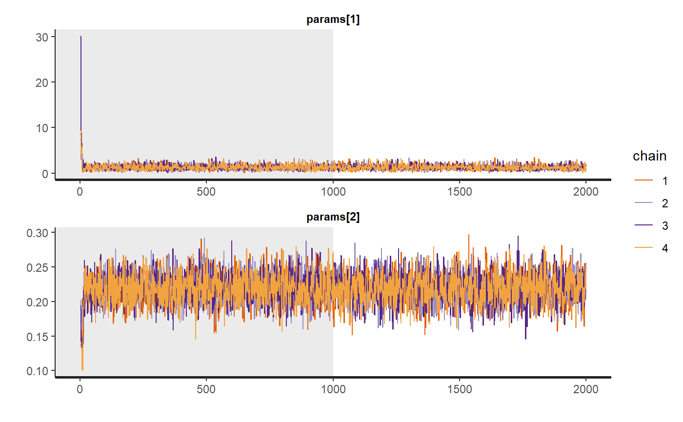
rhats <- bayesplot::rhat(bc_fit$model)
rhats[rhats>1.03]
#> <NA> <NA> <NA> <NA> <NA> <NA> <NA> <NA> <NA> <NA> <NA> <NA> <NA> <NA> <NA> <NA>
#>   NA   NA   NA   NA   NA   NA   NA   NA   NA   NA   NA   NA   NA   NA   NA   NA
#> <NA> <NA> <NA> <NA> <NA> <NA> <NA> <NA> <NA> <NA> <NA> <NA> <NA> <NA> <NA> <NA>
#>   NA   NA   NA   NA   NA   NA   NA   NA   NA   NA   NA   NA   NA   NA   NA   NA
#> <NA> <NA> <NA> <NA> <NA> <NA> <NA> <NA> <NA> <NA> <NA> <NA> <NA> <NA> <NA> <NA>
#>   NA   NA   NA   NA   NA   NA   NA   NA   NA   NA   NA   NA   NA   NA   NA   NA
#> <NA>
#>   NA
bayesplot::mcmc_rhat(rhats)
#> Warning: Dropped 49 NAs from 'new_rhat(rhat)'.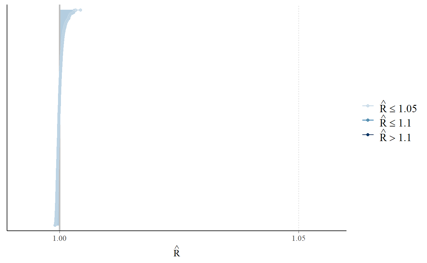
bayesplot::mcmc_nuts_divergence(bayesplot::nuts_params(bc_fit$model),
                                bayesplot::log_posterior(bc_fit$model))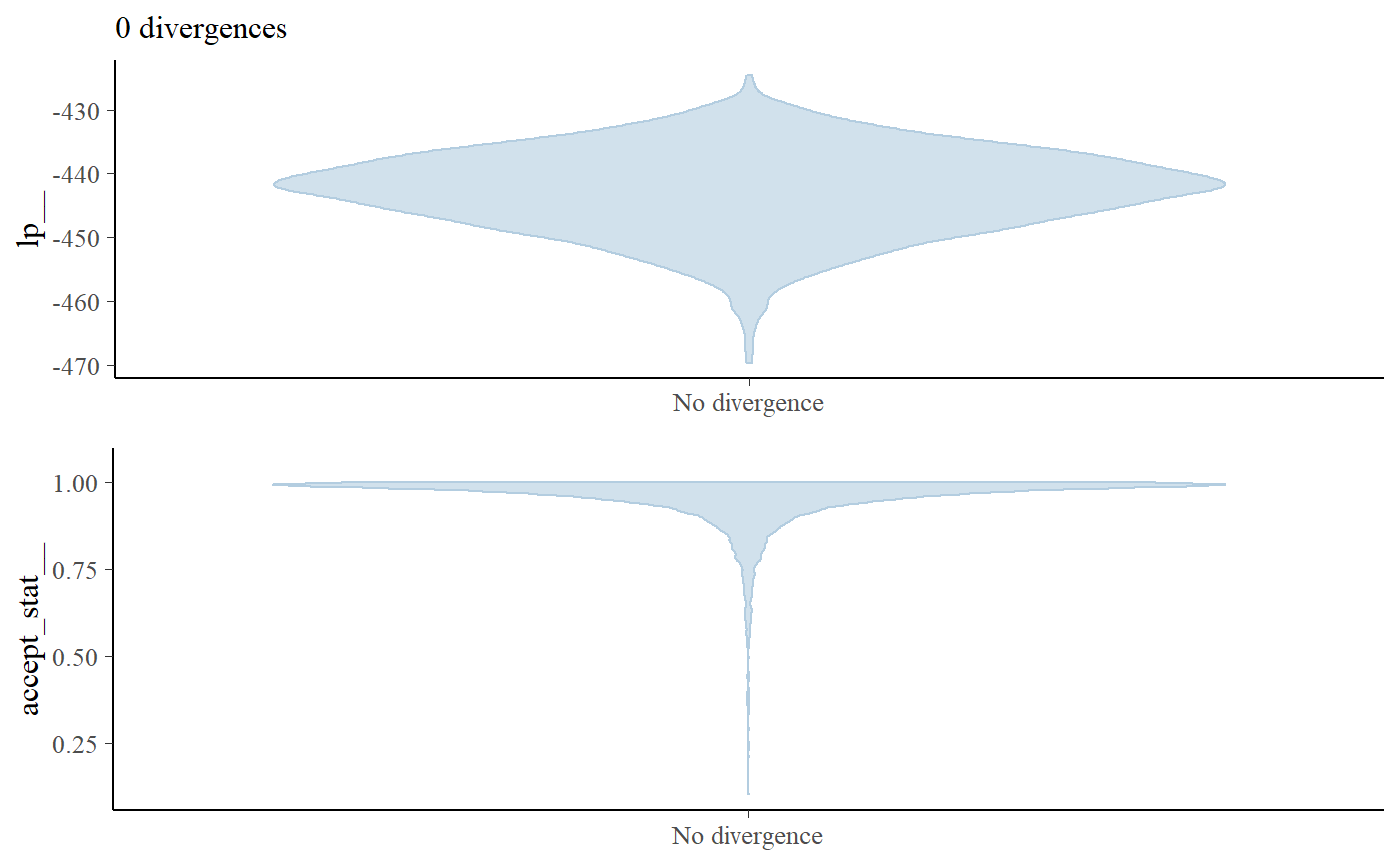
Re-label facilities
Extract the posterior sample and re-label the facilities by their estimated mean \(R_0^k\),
# Extract the posterior samples to a structured list:
posts <- rstan::extract(bc_fit$model)

location_labels <- spread_draws(bc_fit$model,r0k[location]) %>%
  mutate(location = as.character(location)) %>%
  group_by(location) %>%
  summarise(r0 = mean(r0k)) %>%
  arrange(r0) %>%
  mutate(site = LETTERS[1:n()]) %>%
  dplyr::select(location,site)

# get object of incidence and zeta
extracted_posts <- hom_extract_posterior_draws(posts,
                                               location_labels = location_labels)
#> Warning in rpois(dplyr::n(), incidence): NAs produced
Plot model output
result <- hom_plot_r0_by_location(extracted_posts=extracted_posts)
#> Warning: Ignoring unknown parameters: fun.y

# plot results
show(result$plot + labs(y=TeX("$R_{0,k}$")))
#> No summary function supplied, defaulting to `mean_se()`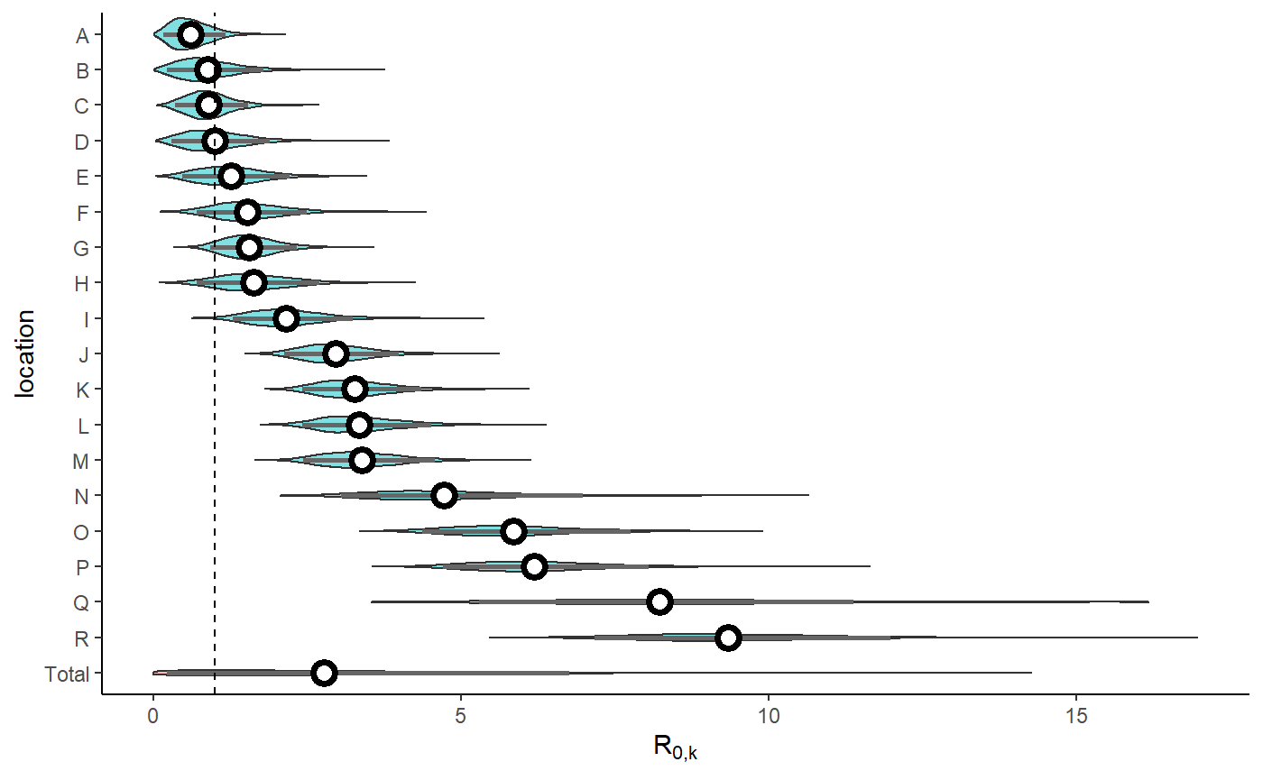
result$table %>%
  kableExtra::kbl() %>%
kableExtra::kable_styling(bootstrap_options=bootstrap_options)| location | r0 |
|---|---|
| Total | 2.29 (0.22 - 6.75) |
| R | 9.17 (7.16 - 11.97) |
| Q | 8.17 (5.29 - 11.38) |
| P | 6.09 (4.7 - 8.04) |
| O | 5.73 (4.37 - 7.76) |
| N | 4.55 (3.05 - 6.98) |
| M | 3.32 (2.43 - 4.58) |
| L | 3.27 (2.42 - 4.51) |
| K | 3.2 (2.41 - 4.35) |
| J | 2.9 (2.13 - 3.98) |
| I | 2.1 (1.29 - 3.23) |
| H | 1.57 (0.7 - 2.69) |
| G | 1.52 (0.91 - 2.33) |
| F | 1.47 (0.7 - 2.5) |
| E | 1.2 (0.46 - 2.21) |
| D | 0.93 (0.3 - 1.89) |
| C | 0.86 (0.35 - 1.54) |
| B | 0.79 (0.22 - 1.79) |
| A | 0.56 (0.16 - 1.17) |
Plot model fit to incidence
result <- hom_plot_incidence_by_location(extracted_posts=extracted_posts,
                                         outbreak_cases = outbreak_cases,
                                         end_time = tmax+5,
                                         location_labels = location_labels)
# plot results
result$plot
#> Warning: Removed 18 row(s) containing missing values (geom_path).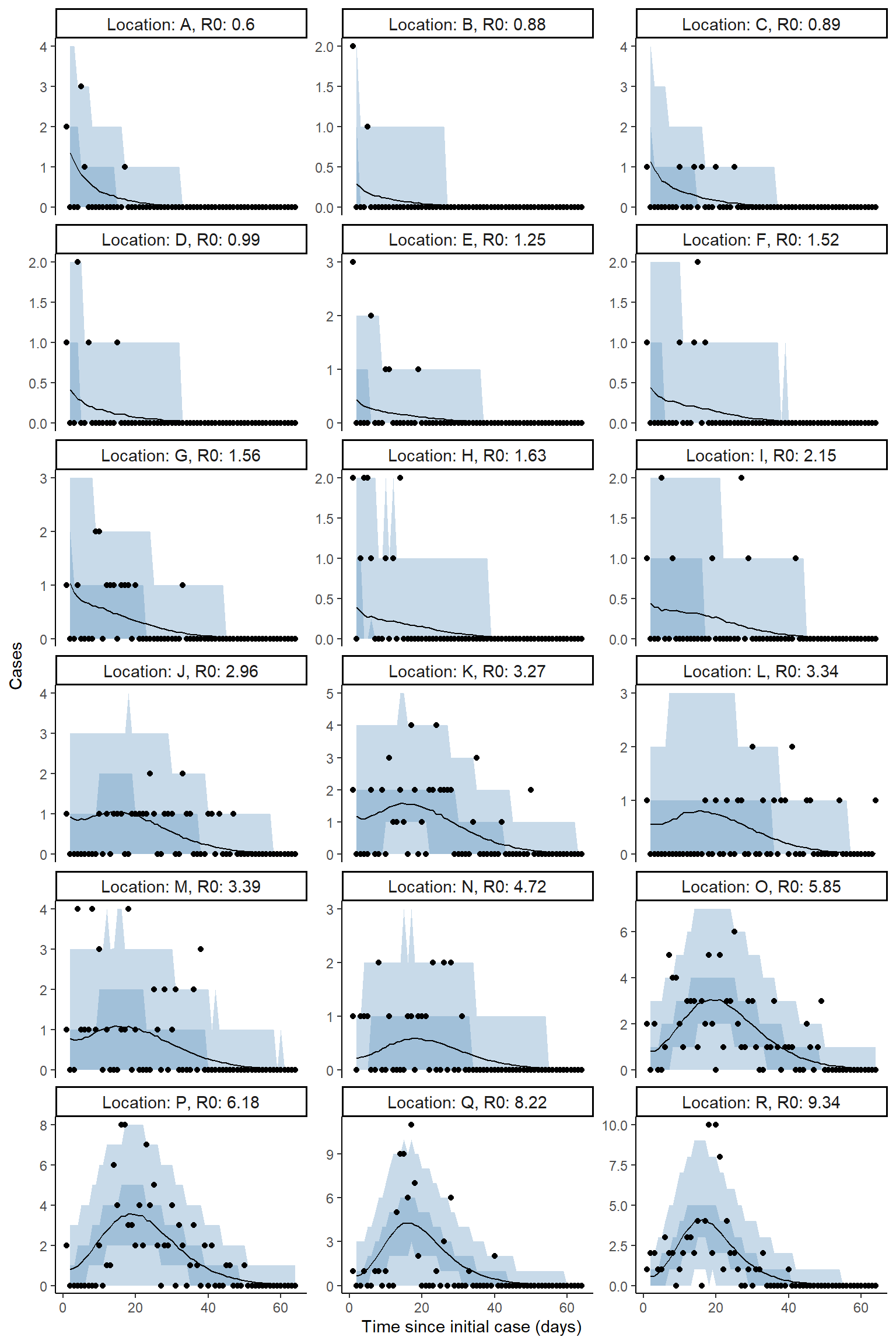
Plot counterfactual scenario
The code below extracts and plots the counterfactual scenario and also provides a summary table of cases by location in the baseline, scenario, where there was no intervention and the difference and proportional difference representing the cases averted. The final row provides a total summary of cases.
result <- hom_plot_counterfactual_by_location(bc_fit,
                                      outbreak_cases = outbreak_cases,
                                      location_labels = location_labels)

# plot results
show(result$plot)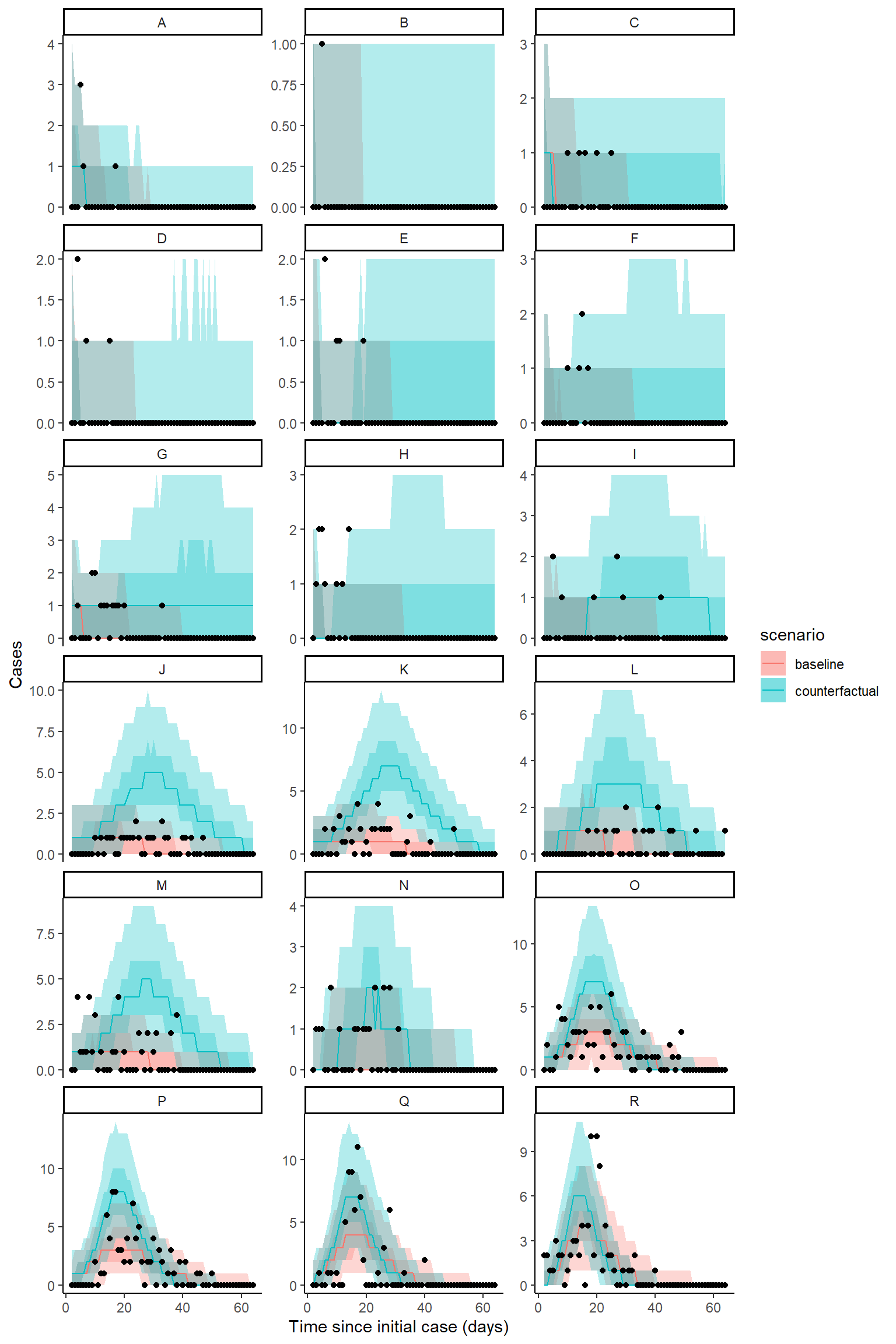
# show table of results
result$table %>%
  kableExtra::kable() %>%
kableExtra::kable_styling(bootstrap_options = c("striped","responsive"))| location | baseline | counterfactual | averted | proportion_averted |
|---|---|---|---|---|
| A | 10 (5 - 17) | 17 (7 - 52) | 7 (-4 - 38) | 0.42 (-0.45 - 0.8) |
| B | 3 (0 - 6) | 6 (1 - 31) | 3 (-2 - 27) | 0.62 (-1.5 - 1) |
| C | 10 (4 - 17) | 23 (8 - 79.05) | 13 (-1 - 67) | 0.59 (-0.14 - 0.87) |
| D | 4 (1 - 9) | 10 (2 - 48) | 6 (-2 - 42) | 0.67 (-0.67 - 0.94) |
| E | 5 (1 - 10) | 18 (3 - 64) | 13 (-1 - 56.05) | 0.75 (-0.17 - 0.94) |
| F | 6 (2 - 12) | 30 (6 - 74) | 24 (2 - 65) | 0.81 (0.29 - 0.94) |
| G | 14 (7 - 23) | 76 (24 - 160) | 62 (12 - 143) | 0.81 (0.5 - 0.92) |
| H | 6 (2 - 12) | 31 (6 - 70) | 25 (2 - 62) | 0.81 (0.25 - 0.94) |
| I | 9 (3 - 17) | 60 (22 - 90) | 50 (16 - 79) | 0.84 (0.67 - 0.93) |
| J | 30 (20 - 44) | 164 (129 - 195) | 132 (98 - 164) | 0.81 (0.73 - 0.88) |
| K | 46 (32 - 63) | 215 (182 - 248) | 168 (134 - 203) | 0.78 (0.7 - 0.85) |
| L | 23 (14 - 35) | 105 (82 - 130) | 81 (57 - 106) | 0.78 (0.66 - 0.87) |
| M | 32 (21 - 46) | 142 (116 - 169) | 109 (82 - 137) | 0.77 (0.67 - 0.85) |
| N | 16 (8 - 27) | 42 (24 - 61) | 26 (4.95 - 46) | 0.61 (0.16 - 0.82) |
| O | 83 (63 - 104) | 142 (117 - 168) | 59 (26 - 91) | 0.42 (0.21 - 0.57) |
| P | 94 (72 - 116) | 148 (123 - 174) | 55 (20 - 88) | 0.37 (0.15 - 0.53) |
| Q | 93 (62 - 118) | 114 (89 - 146) | 18.5 (-12.05 - 77) | 0.16 (-0.13 - 0.55) |
| R | 80 (63 - 100) | 89 (70 - 109) | 8 (-14 - 31) | 0.09 (-0.18 - 0.31) |
| total | 569 (510 - 627) | 1459 (1244.95 - 1735) | 890 (658.95 - 1184.05) | 0.61 (0.52 - 0.69) |
Provide posterior distribution for the proportion of cases averted by location,
show(result$violin_plot)
#> Warning: Removed 151 rows containing non-finite values (stat_ydensity).
#> Warning in regularize.values(x, y, ties, missing(ties), na.rm = na.rm):
#> collapsing to unique 'x' values

#> Warning in regularize.values(x, y, ties, missing(ties), na.rm = na.rm):
#> collapsing to unique 'x' values

#> Warning in regularize.values(x, y, ties, missing(ties), na.rm = na.rm):
#> collapsing to unique 'x' values

#> Warning in regularize.values(x, y, ties, missing(ties), na.rm = na.rm):
#> collapsing to unique 'x' values

#> Warning in regularize.values(x, y, ties, missing(ties), na.rm = na.rm):
#> collapsing to unique 'x' values

#> Warning in regularize.values(x, y, ties, missing(ties), na.rm = na.rm):
#> collapsing to unique 'x' values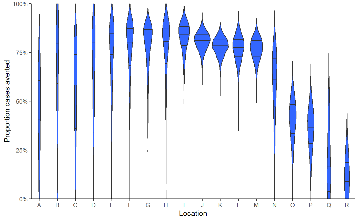
Plot critical times and uncertainty
locations <- BC_LTHC_outbreaks_100Imputs[[100]]$Location
num_cases <- BC_LTHC_outbreaks_100Imputs[[100]]$num_cases
capacities <- BC_LTHC_outbreaks_100Imputs[[100]]$capacity

posts <- rstan::extract(bc_fit$model)


hom_plot_critical_times_by_location(posts,
                                    locations,
                                    num_cases,
                                    capacities,
                                    location_labels = location_labels)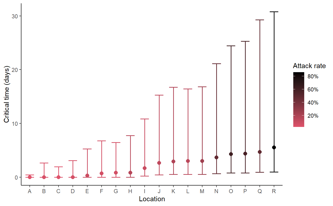
Hierarchichal intervention model
Fit model including estimating intervention by each location in a hierarchical design,
bc_fit_zeta <- seir_model_fit(
  stan_model = stan_mod,
  tmax,n_outbreaks,outbreak_cases,outbreak_sizes,
  intervention_switch = TRUE,
  multilevel_intervention = TRUE,
                       iter = 2000)
Plot model output - zeta model
# Extract the posterior samples to a structured list:
posts <- rstan::extract(bc_fit_zeta$model)

extracted_posts <- hom_extract_posterior_draws(posts,
                                  location_labels = location_labels)
#> Warning in rpois(dplyr::n(), incidence): NAs produced

result <- hom_plot_r0_by_location(extracted_posts=extracted_posts, sort=FALSE)
#> Warning: Ignoring unknown parameters: fun.y

# plot results
show(result$plot + labs(y=TeX("$R_{0,k}$")))
#> No summary function supplied, defaulting to `mean_se()`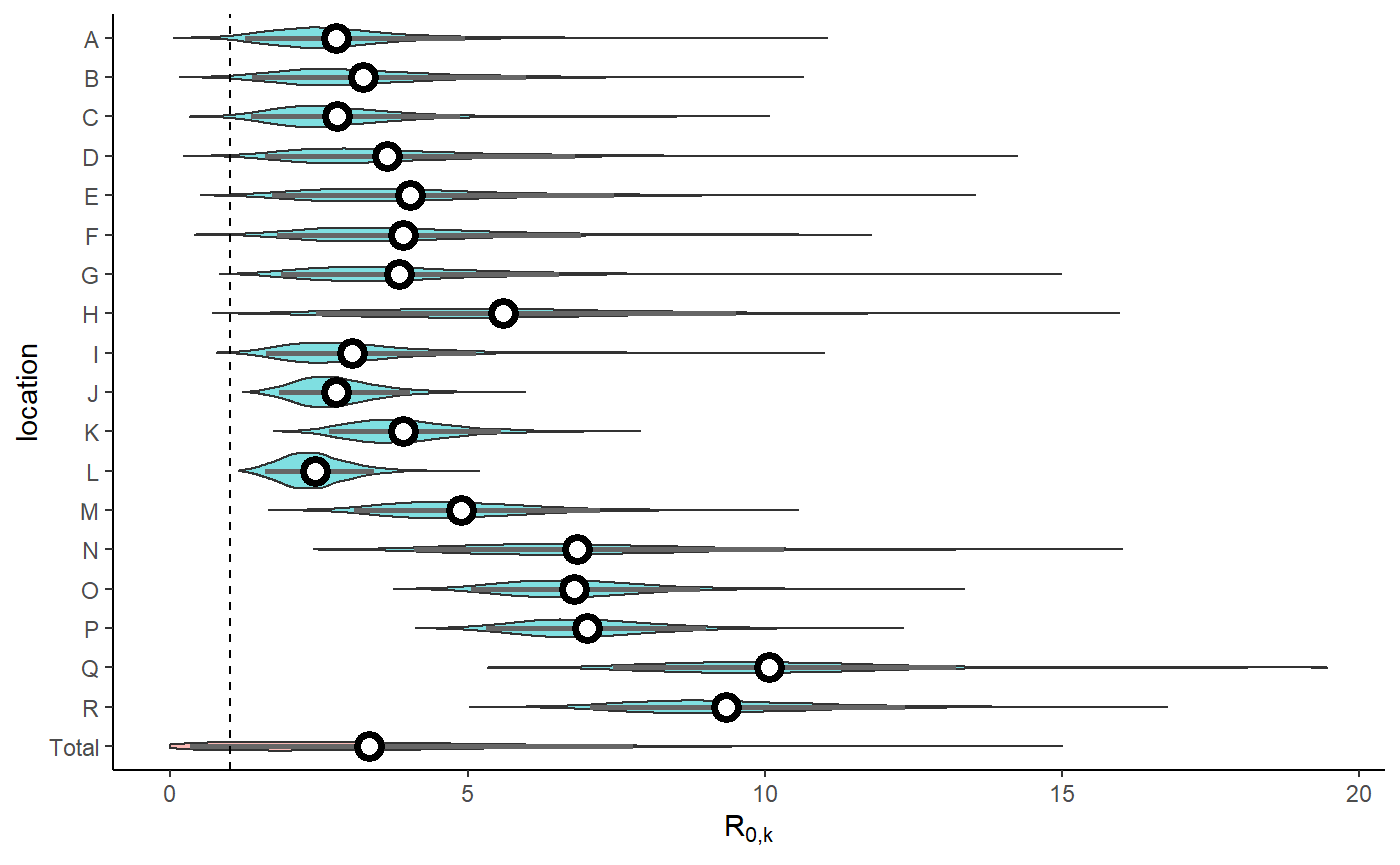
result$table %>%
  kableExtra::kbl() %>%
kableExtra::kable_styling(bootstrap_options=bootstrap_options)| location | r0 |
|---|---|
| Total | 2.96 (0.33 - 7.79) |
| R | 9.13 (7.06 - 12.35) |
| Q | 9.95 (7.44 - 13.21) |
| P | 6.91 (5.31 - 9.01) |
| O | 6.7 (5.06 - 8.9) |
| N | 6.65 (4.1 - 10.32) |
| M | 4.73 (3.08 - 7.23) |
| L | 2.37 (1.6 - 3.43) |
| K | 3.82 (2.67 - 5.55) |
| J | 2.71 (1.83 - 4.03) |
| I | 2.87 (1.61 - 5.14) |
| H | 5.39 (2.45 - 9.52) |
| G | 3.62 (1.85 - 6.54) |
| F | 3.68 (1.8 - 6.9) |
| E | 3.73 (1.7 - 7.46) |
| D | 3.28 (1.59 - 6.81) |
| C | 2.62 (1.35 - 4.87) |
| B | 2.97 (1.38 - 5.99) |
| A | 2.6 (1.26 - 4.96) |
Plot hierarchical intervention strength by location (zeta)
result <- hom_plot_zeta_by_location(extracted_posts=extracted_posts,sort=FALSE)
#> Warning: Ignoring unknown parameters: fun.y

# plot results
show(result$plot)
#> No summary function supplied, defaulting to `mean_se()`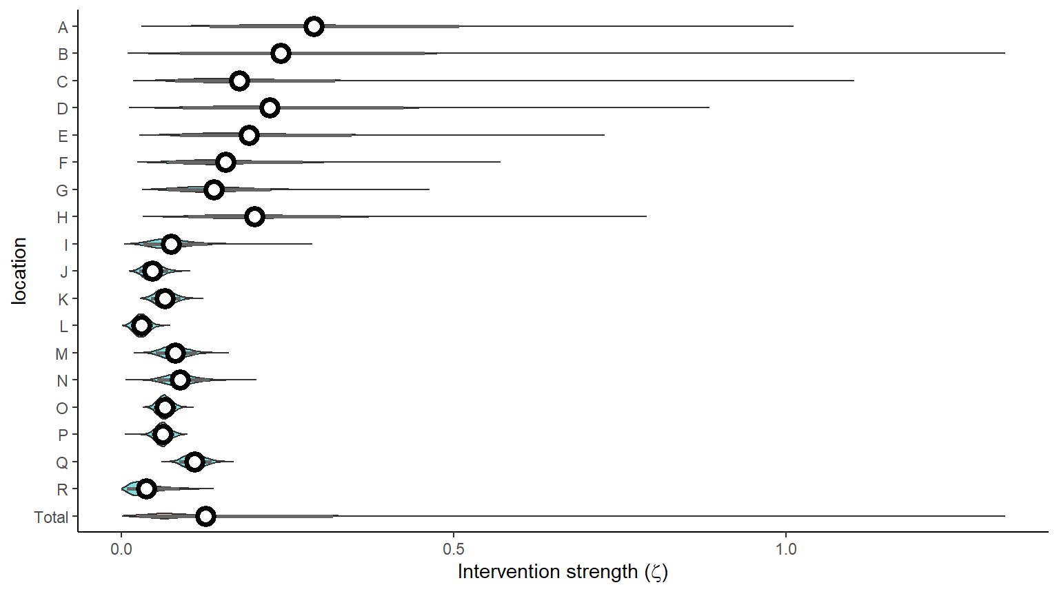
result$table %>%
  kableExtra::kbl() %>%
kableExtra::kable_styling(bootstrap_options=bootstrap_options)| location | zeta |
|---|---|
| Total | 0.1 (0.03 - 0.32) |
| R | 0.03 (0.01 - 0.09) |
| Q | 0.11 (0.09 - 0.14) |
| P | 0.06 (0.05 - 0.08) |
| O | 0.06 (0.05 - 0.08) |
| N | 0.09 (0.05 - 0.13) |
| M | 0.08 (0.05 - 0.11) |
| L | 0.03 (0.01 - 0.05) |
| K | 0.06 (0.04 - 0.09) |
| J | 0.05 (0.03 - 0.07) |
| I | 0.07 (0.03 - 0.13) |
| H | 0.19 (0.1 - 0.33) |
| G | 0.13 (0.07 - 0.22) |
| F | 0.15 (0.07 - 0.27) |
| E | 0.18 (0.09 - 0.35) |
| D | 0.21 (0.09 - 0.42) |
| C | 0.16 (0.08 - 0.32) |
| B | 0.22 (0.09 - 0.46) |
| A | 0.27 (0.13 - 0.51) |
Plot model fit to incidence - zeta model
result <- hom_plot_incidence_by_location(extracted_posts=extracted_posts,
                                         outbreak_cases = outbreak_cases,
                                         end_time = tmax+5,
                                         location_labels = location_labels,
                                         sort=FALSE)
# plot results
result$plot
#> Warning: Removed 18 row(s) containing missing values (geom_path).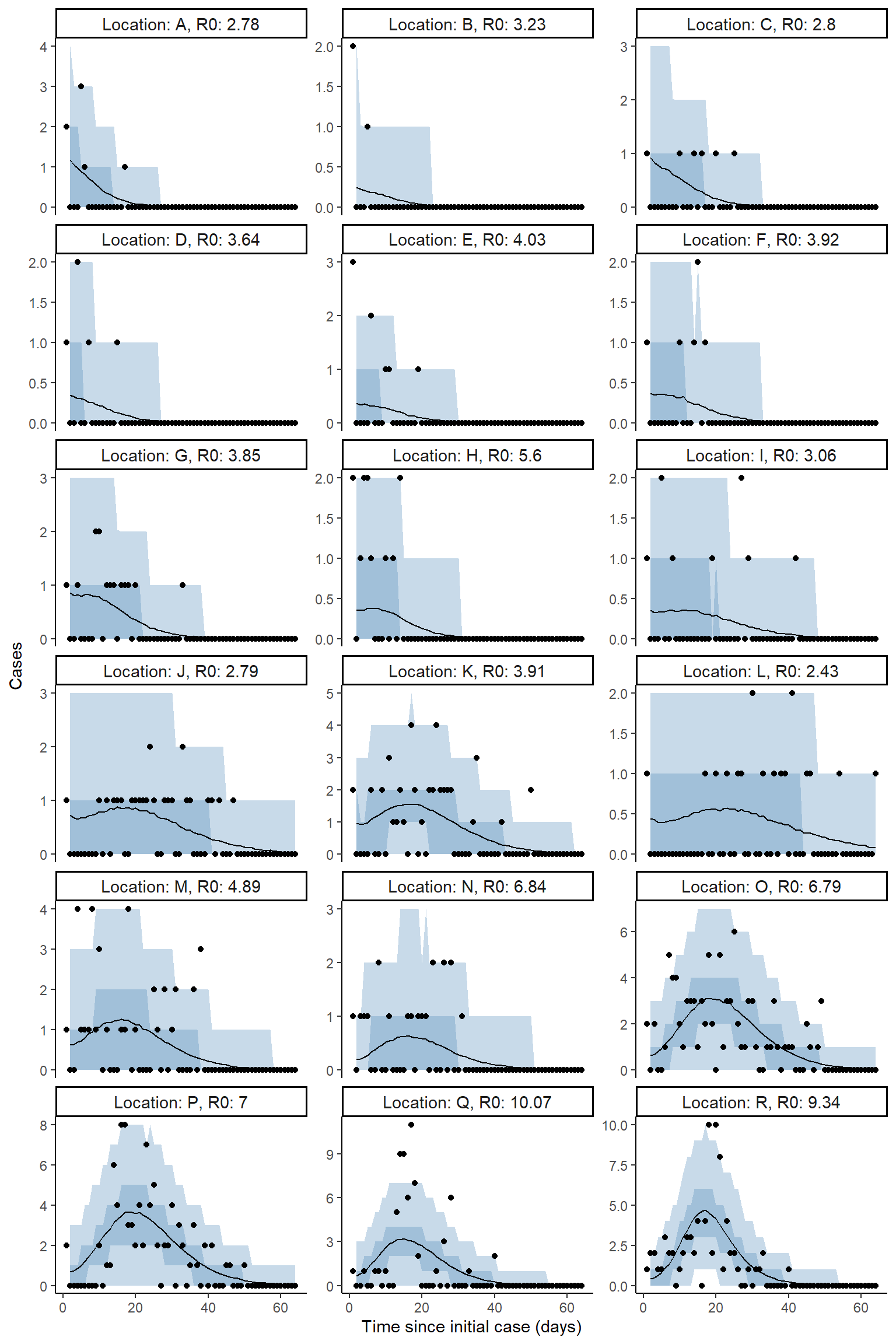
Plot counterfactual scenario - zeta model
The code below extracts and plots the counterfactual scenario and also provides a summary table of cases by location in the baseline, scenario, where there was no intervention and the difference and proportional difference representing the cases averted. The final row provides a total summary of cases.
result <- hom_plot_counterfactual_by_location(bc_fit_zeta,
                                      outbreak_cases = outbreak_cases,
                                      location_labels = location_labels)

# plot results
show(result$plot)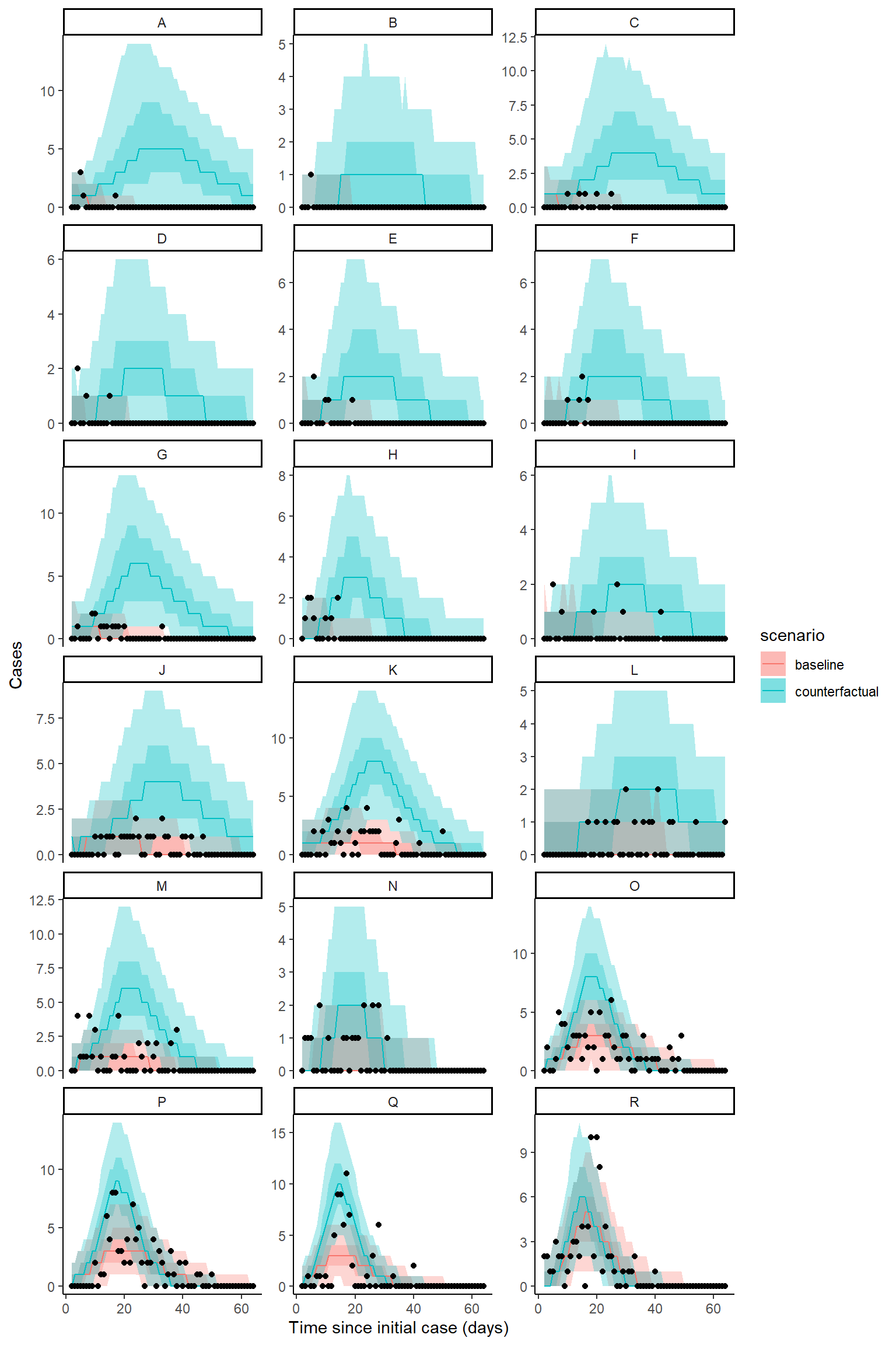
# show table of results
result$table %>%
  kableExtra::kable() %>%
kableExtra::kable_styling(bootstrap_options = c("striped","responsive"))| location | baseline | counterfactual | averted | proportion_averted |
|---|---|---|---|---|
| A | 10 (4 - 17) | 245 (62 - 307) | 235 (52 - 297) | 0.96 (0.84 - 0.98) |
| B | 2 (0 - 6) | 53 (14 - 78) | 50 (12 - 75) | 0.95 (0.83 - 1) |
| C | 10 (5 - 18) | 192 (58.95 - 243) | 181 (48 - 233) | 0.94 (0.82 - 0.98) |
| D | 4 (1 - 9) | 76 (32 - 102) | 72 (28 - 98) | 0.95 (0.86 - 0.99) |
| E | 5 (1 - 10) | 81 (40.95 - 106) | 75 (37 - 101) | 0.94 (0.85 - 0.98) |
| F | 6 (2 - 12) | 83 (43 - 108) | 76 (38 - 101) | 0.93 (0.83 - 0.98) |
| G | 15 (7 - 25) | 193 (111 - 228) | 178 (99 - 213) | 0.92 (0.86 - 0.96) |
| H | 6 (2 - 12) | 76 (53 - 99) | 70 (47 - 93) | 0.92 (0.83 - 0.98) |
| I | 9 (4 - 17) | 74 (34 - 102) | 65 (25.95 - 92) | 0.87 (0.71 - 0.95) |
| J | 29 (18 - 42) | 156 (95 - 194) | 126 (70 - 164) | 0.81 (0.69 - 0.88) |
| K | 46 (31 - 62) | 223 (188 - 255) | 177 (141 - 211) | 0.8 (0.72 - 0.86) |
| L | 23 (13 - 35) | 85 (42 - 116) | 61 (22 - 93) | 0.72 (0.47 - 0.84) |
| M | 33 (21 - 47) | 149 (123 - 176) | 116 (88 - 145) | 0.78 (0.67 - 0.86) |
| N | 15 (8 - 26) | 44 (26 - 65) | 28 (8 - 50) | 0.65 (0.26 - 0.84) |
| O | 82 (62 - 104) | 143 (118.95 - 169) | 60 (29 - 94) | 0.43 (0.23 - 0.58) |
| P | 94 (72 - 118) | 148 (122 - 175) | 54 (17 - 89) | 0.37 (0.13 - 0.54) |
| Q | 67 (49 - 88) | 137 (112 - 163) | 70 (38 - 101) | 0.51 (0.31 - 0.66) |
| R | 83 (64.95 - 103) | 86 (67 - 107) | 3 (-20 - 28) | 0.03 (-0.27 - 0.29) |
| total | 544 (493 - 600.05) | 2225.5 (1756.95 - 2445) | 1681 (1215 - 1909) | 0.75 (0.68 - 0.79) |
Provide posterior distribution for the proportion of cases averted by location,
show(result$violin_plot)
#> Warning: Removed 2 rows containing non-finite values (stat_ydensity).
#> Warning in regularize.values(x, y, ties, missing(ties), na.rm = na.rm):
#> collapsing to unique 'x' values

#> Warning in regularize.values(x, y, ties, missing(ties), na.rm = na.rm):
#> collapsing to unique 'x' values

#> Warning in regularize.values(x, y, ties, missing(ties), na.rm = na.rm):
#> collapsing to unique 'x' values

#> Warning in regularize.values(x, y, ties, missing(ties), na.rm = na.rm):
#> collapsing to unique 'x' values

#> Warning in regularize.values(x, y, ties, missing(ties), na.rm = na.rm):
#> collapsing to unique 'x' values

#> Warning in regularize.values(x, y, ties, missing(ties), na.rm = na.rm):
#> collapsing to unique 'x' values

#> Warning in regularize.values(x, y, ties, missing(ties), na.rm = na.rm):
#> collapsing to unique 'x' values

#> Warning in regularize.values(x, y, ties, missing(ties), na.rm = na.rm):
#> collapsing to unique 'x' values

#> Warning in regularize.values(x, y, ties, missing(ties), na.rm = na.rm):
#> collapsing to unique 'x' values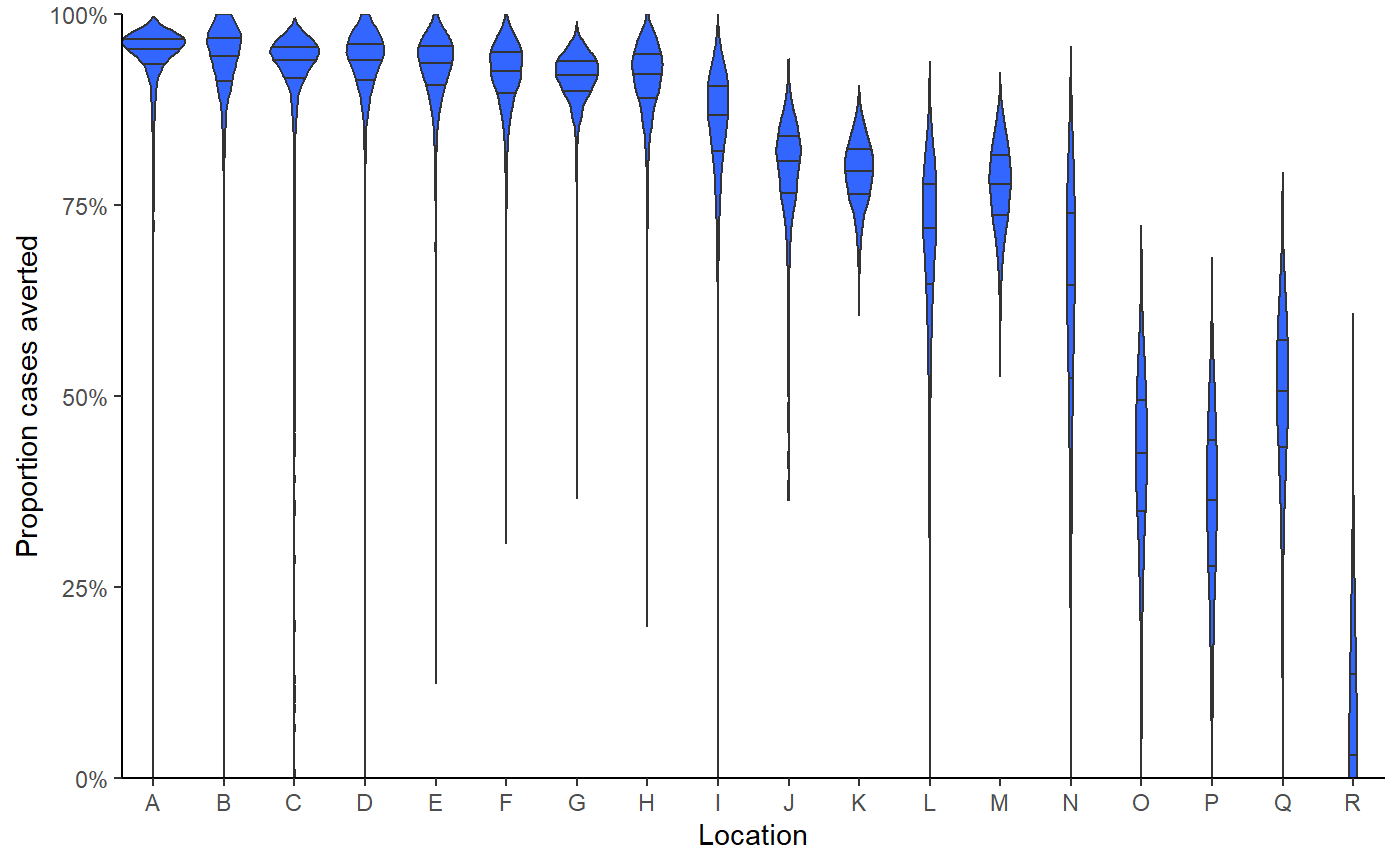
Plot critical times and uncertainty - zeta model
Using the estimates of zeta from the Bayesian hierarchichal model, we estimate the ‘critical time’, that is, the length of time from the introduction of outbreak interventions to R0 dropping below 1, in each facility.
locations <- BC_LTHC_outbreaks_100Imputs[[100]]$Location
num_cases <- BC_LTHC_outbreaks_100Imputs[[100]]$num_cases
capacities <- BC_LTHC_outbreaks_100Imputs[[100]]$capacity

posts <- rstan::extract(bc_fit_zeta$model)


hom_plot_critical_times_by_location(posts,
                                    locations,
                                    num_cases,
                                    capacities,
                                    location_labels = location_labels)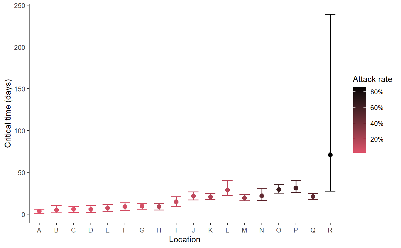
Create parameter comparison table
res <- create_pub_tables(location_labels = location_labels,
                         "Fixed intervention"= bc_fit,
                         "Multiple intervention" = bc_fit_zeta)

res %>%
  kableExtra::kable() %>%
kableExtra::kable_styling(bootstrap_options = "striped")| location | r0 Fixed intervention | zeta Fixed intervention | critical_time Fixed intervention | r0 Multiple intervention | zeta Multiple intervention | critical_time Multiple intervention |
|---|---|---|---|---|---|---|
| A | 0.56 (0.16 - 1.17) | 0.42 (0.07 - 2.29) | 0 (0 - 0.41) | 2.6 (1.26 - 4.96) | 0.27 (0.13 - 0.51) | 3.36 (1.02 - 6.12) |
| B | 0.79 (0.22 - 1.79) | 0.42 (0.07 - 2.28) | 0 (0 - 2.63) | 2.97 (1.38 - 5.99) | 0.22 (0.09 - 0.46) | 4.82 (1.54 - 10.03) |
| C | 0.86 (0.35 - 1.54) | 0.43 (0.07 - 2.12) | 0 (0 - 1.95) | 2.62 (1.35 - 4.87) | 0.16 (0.08 - 0.32) | 5.74 (2.13 - 9.52) |
| D | 0.93 (0.3 - 1.89) | 0.42 (0.07 - 2.23) | 0 (0 - 3.08) | 3.28 (1.59 - 6.81) | 0.21 (0.09 - 0.42) | 5.74 (2.31 - 10.23) |
| E | 1.2 (0.46 - 2.21) | 0.39 (0.07 - 2.3) | 0.28 (0 - 5.25) | 3.73 (1.7 - 7.46) | 0.18 (0.09 - 0.35) | 7.22 (3.29 - 11.88) |
| F | 1.47 (0.7 - 2.5) | 0.41 (0.07 - 2.24) | 0.68 (0 - 6.77) | 3.68 (1.8 - 6.9) | 0.15 (0.07 - 0.27) | 8.78 (4.48 - 13.54) |
| G | 1.52 (0.91 - 2.33) | 0.4 (0.07 - 2.2) | 0.83 (0 - 6.46) | 3.62 (1.85 - 6.54) | 0.13 (0.07 - 0.22) | 9.47 (6.11 - 12.98) |
| H | 1.57 (0.7 - 2.69) | 0.41 (0.07 - 2.19) | 0.81 (0 - 7.75) | 5.39 (2.45 - 9.52) | 0.19 (0.1 - 0.33) | 8.64 (4.95 - 12.96) |
| I | 2.1 (1.29 - 3.23) | 0.4 (0.07 - 2.25) | 1.68 (0.22 - 10.85) | 2.87 (1.61 - 5.14) | 0.07 (0.03 - 0.13) | 14.56 (9.09 - 20.85) |
| J | 2.9 (2.13 - 3.98) | 0.4 (0.07 - 2.35) | 2.63 (0.44 - 15.25) | 2.71 (1.83 - 4.03) | 0.05 (0.03 - 0.07) | 21.48 (17.12 - 26.62) |
| K | 3.2 (2.41 - 4.35) | 0.41 (0.07 - 2.25) | 2.89 (0.5 - 16.74) | 3.82 (2.67 - 5.55) | 0.06 (0.04 - 0.09) | 20.69 (17.47 - 24.48) |
| L | 3.27 (2.42 - 4.51) | 0.39 (0.07 - 2.18) | 3 (0.52 - 16.42) | 2.37 (1.6 - 3.43) | 0.03 (0.01 - 0.05) | 28.8 (22.29 - 40.08) |
| M | 3.32 (2.43 - 4.58) | 0.4 (0.07 - 2.3) | 2.99 (0.51 - 16.82) | 4.73 (3.08 - 7.23) | 0.08 (0.05 - 0.11) | 19.55 (16.13 - 23.83) |
| N | 4.55 (3.05 - 6.98) | 0.42 (0.07 - 2.31) | 3.67 (0.65 - 21.14) | 6.65 (4.1 - 10.32) | 0.09 (0.05 - 0.13) | 21.72 (16.67 - 30.56) |
| O | 5.73 (4.37 - 7.76) | 0.41 (0.07 - 2.21) | 4.29 (0.81 - 24.44) | 6.7 (5.06 - 8.9) | 0.06 (0.05 - 0.08) | 29.28 (25.18 - 35.4) |
| P | 6.09 (4.7 - 8.04) | 0.41 (0.07 - 2.25) | 4.39 (0.8 - 25.29) | 6.91 (5.31 - 9.01) | 0.06 (0.05 - 0.08) | 31.01 (26.26 - 40.06) |
| Q | 8.17 (5.29 - 11.38) | 0.44 (0.07 - 2.21) | 4.7 (0.92 - 29.29) | 9.95 (7.44 - 13.21) | 0.11 (0.09 - 0.14) | 20.94 (17.89 - 24.51) |
| R | 9.17 (7.16 - 11.97) | 0.4 (0.07 - 2.3) | 5.54 (0.96 - 30.79) | 9.13 (7.06 - 12.35) | 0.03 (0.01 - 0.09) | 70.87 (27.63 - 239.34) |
| Total | 2.51 (0.47 - 9) | 0.41 (0.07 - 2.24) | 1.49 (0 - 16.67) | 4.07 (1.76 - 10.06) | 0.1 (0.03 - 0.32) | 16.95 (3.05 - 41.83) |